
The main objectives of this assignment are to take a procedurally generated SLIDE model from the folder http://www.cs.berkeley.edu/~sequin/CS184/AS9_SCU/ and provide this model with suitable surface definition or texture, then illuminate it properly with two or more light sources, choose a viewing angle that brings out the model's best features; and then use a more sophisticated rendering system than SLIDE can offer to produce a high quality rendering of the given object. In order to use a more powerful rendering system, you must generate a RIB output file, which you can then render with BMRT. The procedural models used in this assignment will need to include a new surface property called texture. You will use the rendering system to produce a series of images highlighting various visual effects, including shadows, radiosity (color bleeding), antialiasing, and area lights. These images along with a brief write-up will be your submission. See the references section for links to other pages and informative sections from your text book.
A bit of caution: Do not waste time rendering high resolution images with radiosity until you are almost done! Instead, concentrate on getting your geometry, surface properties, light positions, and viewing parameters optimized. This will make your work much more efficient. Do not forget to read the summary of how to start section at the end of the document.
This is your chance to show that this semester's 184 class can produce great displays. We will post a few of the most interesting images when the assignment is complete!
Procedural modeling is an algorithmic way of producing geometric data. For this assignment we will give you a few SLIDE files with geometrical shapes that might make impressive constructivist sculptures, if they are built at the right scale, from the right materials, placed on a proper pedestal, and properly illuminated. You find these sculpture models in http://www.cs.berkeley.edu/~sequin/CS184/AS9_SCU/ . To find the best possible presentation for one of these models is your assignment! Thus, this assignment is primarily about textures and lighting and rendering; the generation of geometry is somewhat secondary for now -- you can then fully let your creativity roam in that respect during the final project. Thus a first key decision is to choose a suitable texture. Look at the geometry of the piece that you chose, and ask yourself would this be implemented best in stone, or in metal, or in glass ... Then you may have to add texure coordinates to your vertices, and textures to your surfaces to make your object more interesting. Texturing is discussed in more detail in the section on texture mapping. If you want to refine or enhance the basic geometry given, you may want to use a tclinit block to generate that more sophisticated geometry with the extra information for the renderer. The full version of SLIDE that you will use for this assignment knows how to process this tclinit block.
In addition to standard geometry, your procedural model will also include surface properties, such as color, diffuse and specular coefficients, and also texture information. The idea of texture mapping is to repeatedly paint the same small picture onto your geometry. The motivation is to efficiently model intricate patterns that would require a great deal of very small geometry information. In SLIDE each point can also specify a texture coordinate, and a surface contains the name for a texture file. For SLIDE your texture file must be a .gif file, and the height and width in pixels must each be a power of 2. On the PC, Microsoft Imaging editor or some other utility should let you convert images from other formats. On UNIX xv can do this for you. In SLIDE you will specify a texture file for each textured surface. If a surface is to be textured you should probably set its color to ( 1 1 1 ) because SLIDE multiplies the surface color by the texture map values. The next step is to specify texture coordinates for each vertex of the faces in your surface. When the texture map is applied, the renderer linearly interpolates the texture coordinates you supply to obtain a coordinate for a particular point on the surface. The texture mapping algorithm then samples the texture at the coordinates obtained and uses that value to color the pixel. The following figure gives some examples.
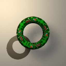
Texture coordinates are usually two values (s and t) but SLIDE requires three values and ignores the third. The geometric coordinates in the diagram are in 2D, but for SLIDE (as you know!) they are in 3D. Read the SLIDE language description and your textbook for more more details. The tricky part about texture mapping an object consisting of multiple polygons is assigning texture coordinates so that the texture is smooth and continuous over the object. There are some tricks to this. One is to use a texture with a solid background color and some seperated foreground elements (stars on black or random polka dots are examples) then it is easier to get away with approximating continuity. The torus.tcl file shows a good example of how to wrap a texture around an object smoothly. Note that the circuit board texture we use for the torus is tileable, which means that if you put a bunch of copies next to eachother there are no disconituities in the texture. This and the wood texture both came from this site. Note that while all of the textures on that site tile, many are not a power of 2 by a power of 2 in size, so you will have to resize them in an image editing program.
Radiosity methods allow the computation of illumination due to light that bounces off of multiple diffuse objects along its path from the light source to the viewer. Since most objects are modeled as having a diffuse coeficient and a specualr coeficient, we usually see multiple "diffuse bounces" off of objects. Ray-tracing by itself only models light that makes one diffuse bounce and then multiple specular bounces on its way from the light source to the viewer.
In order to compute the effect of diffuse light bouncing off of objects, we break the scene down into small facets on all the surfaces. We assume the facets are lambertian surfaces and that they are small enough so that light striking them from a nearby light source is coming in at the same angle over the entire facet (note this is not true for a large polygon!). Then we compute how much light reaches the diffuse surfaces directly from light sources. As discussed earlier, a diffuse surface patch under illumination looks like an area light source, so in the next step we treat all the illuminated diffuse patches as light sources, and once again calculate how much light falls on each of the diffuse patches. Ideally we would repeat this calculation a very large number of times, summing the light directly from the light source, from one bounce, from two bounces, etc... To do this would require computing the powers of a large matrix describing how much light travels from each facet to each other facet. If our scence had say one million facets this becomes a million by a million matrix, and is difficult to raise to a power! In practice people estimate the effects which will appear brightest in the image. For your .rib files you can help the radiosity renderer, by telling how big to make the facets for your scene. If it breaks your scene up into too many small facets, the rendering time will be very long! On the other hand if it breaks your scene up into too few facets, the illumination will be be clearly wrong.
Antialiasing depends heavily on ideas from signal analysis, and sampling theory, but for our purposes in this assignment we will take a simple approach to the subject. The goal of antialiasing is to remove artifacts of sampling from the image. In this case the problem is sampling only one color value per pixel. This results in what has come to be known (it's actually in the dictionary as a computer graphics term) as the "jaggies" or the staircase-like effect along the edges of lines or polygons in an image. One solution to this problem is to color a pixel based on the percentage of its area covered by a polygon. This is called "unweighted area sampleing". An example of the normal technique next to an example of unweighted area sampling follows:
 While analytically computing the area of this intersection would be
difficult, especially in a ray tracing system, there is a more
straightforward way to get an approximation of this result. By
sending out a large number of rays through a pixel and averaging their
color values, we get an approximation to area weighted sampling. The
following image shows a number of rays (the black circles) sent out in
the direction of a pixel. The color of the pixel is determined by
the average of the color of the surface each ray hits.
While analytically computing the area of this intersection would be
difficult, especially in a ray tracing system, there is a more
straightforward way to get an approximation of this result. By
sending out a large number of rays through a pixel and averaging their
color values, we get an approximation to area weighted sampling. The
following image shows a number of rays (the black circles) sent out in
the direction of a pixel. The color of the pixel is determined by
the average of the color of the surface each ray hits.
How do I get a RIB file?
From the SLIDE viewer you can output a RIB file of the current
geometry by selecting "save as rib" from the file menu. For
this
assignment you will be using the full SLIDE viewer called
slide which has all the features of SLIDE implemented for
you. Once you have written the RIB file (name it with extension
.rib), quit slide. You can examine the RIB file in a
text editor, it is basically a tagged text file. The RIB files
produced by the SLIDE viewer have comments that should help you find
which parts of your geometry have been converted into which parts of
the RIB file. The RIB file will contain information about geometry,
surface properties, and light sources. While RIB supports texture
mapping, it cannot use the .gif files that SLIDE does. At the end of
the RIB file produced by SLIDE there will be a list of the texture
files
used in the file. You need to convert each of these from a .gif file
to a .tif file, and then to a .tx (texture) file. You can use
microsoft imaging editor (under accessories on the nt machines in
the lab) to produce .tif files from your .gif file. Load the .gif and
then select "save as". Be sure to save the file as a 24 bit
tiff (this
is an option under "more" in the save as dialog), otherwise it will
not work. Follow the instructions from the next step for setting the
path to the BMRT binaries, and then you can run the following command
to convert your tiff into a texture file:
T:\mkmip.exe myTexture.tif myTexture.tx (for BMRT)
T:\texmake myTexure.tif myTexture.tx (for Pixie)
This will produce a file called myTexture.tx which you should place in the same directory as the RIB file. Once you have done this for all the textures you are using, you are ready to begin rendering!
We are supplying two RIB compliant renderers: Pixie and BMRT. You are also free to use other renderers, such as Maya.
Using Pixie will probably be slightly more of a hassle, but what you will learn is more useful. For standard features, Pixie uses the same interface as Pixar's Renderman (the Renderman Interface). This will give you practice editing rib files and get you somewhat acquainted with some things that people actually do, including writing shaders.
Pixie is setup on the labs already. If you download Pixie for windows (http://www.cs.berkeley.edu/~okan/Pixie/download) at home, there will be a couple of environment variables to change.
Add "C:\Program Files\Pixie\bin" (or wherever the bin folder is on
your machine) to you path
Add a new environment variable called "PIXIEHOME" and point it to
"C:/Program Files/Pixie"
(or wherever Pixie is)
When you render the .rib file straight from SLIDE, you'll notice that there are no shadows. This is a good first thing to fix. You must (1) add lines to the .rib file and (2) create a custom shader that takes visibility into account.
SHADOWS:
To turn on ray tracing (for shadows, etc.) add this to the beginning of
the .rib file:
Attribute "visibility" "trace" [1]
Attribute "visibility" "shadow" [1]
Attribute "visibility" "transmission" "opaque"
Once the raytracing is turned on, you can use visibility(A,B) to
compute
shadows inside light source shaders or trace(A,B) inside the surface
shaders.
For example, to make pointlight shader cast raytraced shadows, change
the
shader from
illuminate (from) {
Cl = intensity * lightcolor / (L . L);
}
to
illuminate (from) {
Cl = visibility(from,Ps)*intensity * lightcolor / (L . L);
}
Also change the name of the shader in the file from 'light' to 'mylight' for example.
Save your changed shader in your as9 folder (perhaps a /shader subfolder).
You will then need to recompile the shader that you've
changed.
At the command line, in the directory containing the .sl file:
sdrc myshader.sl
This should create mylight.sdr (following from my example)
Note that even if you change pointlight.sl and save it as
pointlight2.sl, when you compile it, it
WILL
OVERWRITE pointlight.sdr INSTEAD of generating
pointlight2.sdr. The shader name is the name
in the
file not the filename.
Now you'll have to replace the previously named light shader in the
.rib file
'light' to your new shader 'mylight'. Also, you'll have to add a
line to
add your shader directory to its shader searchpath.
Option "searchpath" "shader" "H:/myshaders:&"
Now rendering the .rib file should produce an image with shadowing.
That's sort of a lot to get shadows working, but these are exactly the same issues you would face using Pixar's Renderman.
AREA LIGHTS:
You shouldn't actually have to do anything for area lights, but you may
want
to tweak the parameter. This line that SLIDE already places in
the RIB
file for you is:
Attribute "trace" "numarealightsamples" [30]
30 is a pretty good number, but a higher number will give you a smoother result.
PHOTONMAPS:
Pixie does not implement radiosity. It uses Photon Maps which are more
useful in generating all aspects of global illumination (not just
diffuse bounces).
Normally a modelling package, like Maya, will have options to add lines
for
irradiance caching to the rib file for you. It will format your
file to do
fancy things like a two pass rendering. That will be difficult for you
to
do by hand so we're going to try and stick with one pass.
RIB file changes:
Option "hider" "photonmap" [1]
Attribute "visibility" "photon" [1]
Attribute "trace" "maxdiffusedepth" [1]
Note that global illumination is a messy process and involves lots of
parameter tweaking. The parameters involved in photon mapping and their
default values are:
Attribute "globalphoton" "estimator"
[100] # the number of photons to use in
radiance estimate
Attribute "globalphoton" "maxdistance" [1] #
The lookup distance
Attribute "globalphoton" "emit"
[10000]
# Number of photons to emit
Option "irradiance" "maxerror"
[0.5]
# The irradiance cache error control
Option "irradiance" "minsampledistance" [0.1] # The irradiance
cache error control
Option "irradiance" "maxsampledistance" [1] # The
irradiance cache error control
You can use causticphoton instead of globalphoton above.
Okan was nice enough to fiddle with the parameters and find what looks good for one of the example scenes. They are these. Try them first when you're looking at photon maps:
Attribute "globalphoton" "estimator"
[500]
Attribute "globalphoton" "maxdistance" [1]
Attribyte "globalphoton" "emit" [100000]
Also you must change all instances of the "plastic" and "matte" shader to "gplastic" and "gmatte" respectively
The Pixie documentation can be found online at http://www.cs.berkeley.edu/~okan/Pixie/doc/">.
You may also find it useful to browse through the complete PIXAR Renderman Interface Specification
You can download the Win32 binaries for BMRT
here. If you need it for other platforms, email the TA's.
The first step of rendering is to setup some environment variables so that you can easily run the BMRT utilities from the dos command prompt. The software is installed on the caffe partition, and you will need to add some entries to your path and some environment variables. To do this right click on the My Computer icon in the upper left of you windows nt desktop, and select the environment tab.
For your path add the following directory:S:\bmrt\SYSTEM\NT\bmrt2.4\binThen add the following two environment variables with the values shown:
SHADERS
S:\bmrt\SYSTEM\NT\bmrt2.4\shaders
HOME
S:\bmrt\SYSTEM\NT\bmrt2.4
rgl.exe shadtest.ribThis should produce a faint image. Then try:
rendrib.exe -d shadtest.ribThis should produce a more detailed image. Now you are ready to go to the directory with your .rib RIB file and .tx texture files and render away. Near the beginning of a SLIDE produced RIB file is a line beginning with
Display. The first argument in quotes is the name of the
file the rendered image will be saved to if you save it. The next
argument tells the renderer to render to the screen. Once the image
has been rendered to the screen you can press "w" in the viewing
window and it will be saved to the filename specified. The output is
always a TIF file, and should have extension .tif. Also near the
beginning of the RIB file is a line beginning with
Format with two parameters that specify the size of the
output image in pixels. You can make this smaller to speed up
rendering. I suggest commenting it out completely and using the -res
command line option described below. The following command line
options for rendrib.exe will probably be usefull while you render
various images.
| Command Line Option | Description |
| -samples a b | Makes the ray tracer send out a columns of b rays per pixel for a total of ab rays per pixel |
| -var threshold min max | Sends out min samples per pixel, if these samples have a variance above threshold then send out up to max samples until the variance is below the threshold. |
| -d [n] | Tells BMRT to render to the screen. The optional argument n makes it trace each nth line creating a progressive refinement of the image. (Good for a quick check.) When the rendering is done, pressing w in the display window will save the .tif file, if one was specified in the .rib file |
| -res x y | Tells BMRT to make an image x by y pixels in size. |
| -radio n | Tells BMRT to use radiosity and compute at most n radiosity passes. |
You can find more information in the README files in the BMRT installation (see Links and References below).
You will need to hand in some code, a .rib file, a sequence of five
images and three short write-ups as follows:
Put your four write-ups in a file called ANSWERS,
and each one of your images in a file named "image[1-5]xx.jpg",
where the "xx"-part represents the letters of your instructional
account.
Then submit all of these files from your as9 directory.
You may do this assignment alone or with your preferred partner;
but if you work as a pair you will have to submit twice as many images:
labeled as "image[1-5]xx.jpg" and "image[1-5]yy.jpg", respectively,
reflecting your two account logins.
You may use the same sculpture model and the same basic setup,
but you should choose two different sets of materials, surface
treatments,
light constellations, and viewpoints.
Rendering 1
Select one of the sculpture models, perhaps add a pedestal and some
simple environment
(a "lawn" or a "pond" and/or a background facade ...). Pick some lights
in proper places and a good camera position, that makes the sculpture
look as good as possible. Create an image
called image1xx.jpg in jpeg
format of this whole set-up rendered in SLIDE. On Windows NT
"control"+"Print Scrn" copies the active window to the clipboard. You
can then open Microsoft Imagining editor and select new image from
selection to make an image file with your window. Save this as a .jpg
with less than 10% compression (quality factor 90% or greater), as
this will make the image reproduction accurate enough to see clearly.
This image should have all the same light sources that your other
renderings have (except that any area light sources are reperesented
just with point lights).
This rendering will clearly have an un-natural harsh
"computer-graphics" look
with al lack of realistic shadows.
With the subsequent renderings you should try to improve that situation
as much as possible.
Write-up 1
List the modifications you made to the supplied model source code.
Describe the additional elements added to complete the scene,
and the number and positions of the lights ( at least one of them
should be an area light!).
You might want to include a diagram (diagram.jpg)
if this makes things easier to explain/understand. Note that this
desciption is crucial for the readers to understand what you are trying
to do
and will almost certainly affect your grade. It is in your best
interest
to invest more than a couple minutes making it clear and concise.
Rendering2
Now render your scene with Pixie or BMRT. This rendering
should use the same light sources as the above image, and should be
from essentially the same viewpoint. Try to make as many improvements
in the lighting condition as possible, and keep track of the
differences between the two images. Keep them the same image size in
pixels,
(which should happen by default), so that you can more clearly see what
differences the two different renderers make. This will also help with
the next part of the
assignment. You will need to convert the output of bmrt (.tif) to a
jpeg file, call it image2xx.jpg (Microsoft Imaging editor
will do this, again 10% or less compression)
Write-up 2
List the differences that you observe between the two different
renderings of your scene done by Slide and by Pixie. For
each difference, point out where in the image the difference is most
visible
and briefly explain what you think causes that difference.
( For example, it might have something to do with antialiasing.) If you
play
with the "-samples" option described above, you should be able
to produce nice antialiasing in your output.
Also discuss how the number of samples affects renderings comprising
an area light source. Describe what happens when the
number of samples is too small, and why. You should try to be concise
and concentrate on the best answer. You should definitely consult any
references you can find; and it is OK to discuss the generic high-level
issues with your friends and colleagues! Again you will be receiving
credit for your answers, so it is worthwhile to do your write-up
carefully.
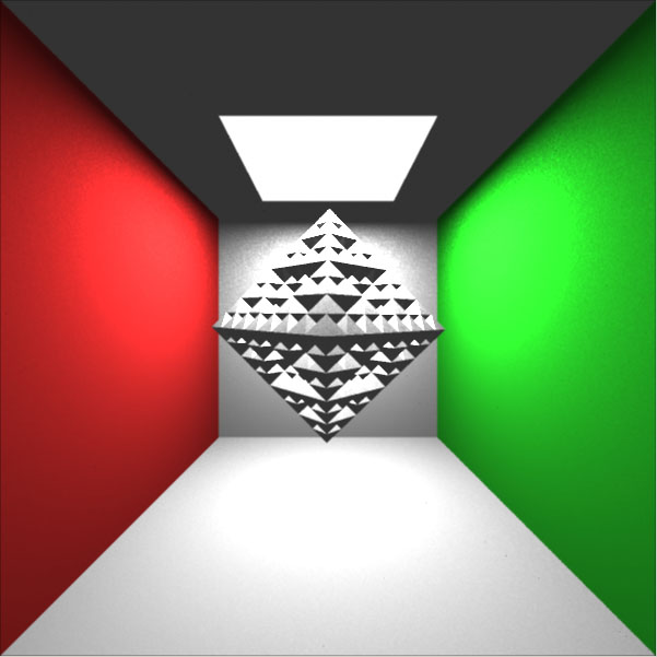
Renderings 3 and 4
Renderings 3 and 4 will mimic "indoor" scenes -- something like a scene
in a museum.
Place your chosen model inside a room (you might think of it
as an inside out box) with light grey walls and a texture mapped
wood floor (DO NOT use the wood texture from our example, find your
own!).
Place area light sources on the walls and/or ceiling to
illuminate the scene. Then render first without radiosity and then with
radiosity. Your rendering should display color bleeding, and other
radiosity effects (you can read about these in your textbook). Again,
convert both output files to .jpg format. Name the one without
radiosity image3xx.jpg and the one with radiosity image4xx.jpg
Write-up 3
Write a short discussion of the radiosity effects, in particular, how
are they
different from just using area light sources in the same scene.
Rendering 5
Make one final "publishable" rendering -- indoor or outdoor, whatever
you think works best for the sculpture you have chosen.
For this rendering you may choose somewhat different materials or
textures,
if from the above experiments you have learned what works well and what
does not.
For the indoor scene, you may now put wall-paper texture onto the
walls, etc ...
But keep in mind, showing off the sculpture is the essential thing and
the
focal point of this display.
The best of these final renderings may get used in forthcoming conferences and/or publications -- of course with proper credit to the originator.
No write-up needed for this image -- it should speak for itself.
Okay, so you are ready to make insanely great models and
renderings.
This section will step you through getting started.
NOTE: SLIDE seems to crash everytime we save anything with a procedural
texture (e.g. torus) as a RIB file. Since the steps below rely on
having a working RIB file, we have created a separate tutorial to help
you get started. You can
access it here.
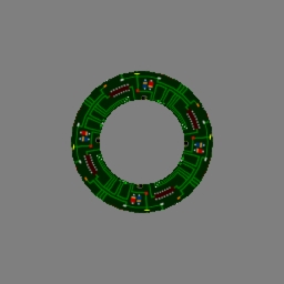
slide. All of the demo files
are available in as9.tar.gz. Copy the files
into your own directory. Run SLIDE from that directory, and load torus_simple.slf.
This file is a demonstration of
procedural modeling. It is heavily documented and relatively simple
(only sources the torus.tcl file, references the comp005.gif
texture, and otherwise it stands on its own)
so you can read through it to see what is happening. You can use the
built in crystal ball interface to rotate the scene around to see a
torus texture mapped with circuitry in front of a background plane.
When you are ready, go to the file menu and select save as rib. Note
that the position of the built in crystal ball will not effect the
orientation of the .rib file output. Later on if you use a .tcl
crytstal ball interface (see torus.slf and disable the
crystal ball interface by pressing the "u" key) that actually changes
a tranform in your hierarchy, then that will affect the rib file
produced. Slide will then bring up a dialog, where you should name
your rib file torus_simple.rib. At this point you should
probably quit
SLIDE to conserve system resources. mkmip.exe comp005.tif comp005.txand make sure that the .tx file is in the current directory with torus_simple.rib. Now we can make a pretty image! To do this type
rendrib.exe -d 16 torus_simple.ribat the command line. This will produce an image on your screen. You should be able to see some differences between this and the SLIDE rendering of the scene, but they are slight because we are only using an ambient light source. Pressing w in the viewer will write a tiff file with the name specified in .rib file near the beginning on a line starting with
Display. You can change that name to
whatever you
want. You can quit the viewer with q or esc.
 |
| torus_simple.tif : Ambient Light |
arealight alCeilingLightHere is the definition in SLIDE for an area light source. The color is so large because it actually encodes the amount of energy coming from the light source. You also need to add an arealight path instead of a light path to your render statement like so:
color ( 80 80 80 )
instance oSquare
rotate ( 1 0 0 ) ( 180 )
endinstance
endarealight
arealight gWorld.iAreaLight.alAreaLightNow look at the scene in slide. The glowing light above the torus (visible from the torus' perspective) is an approximation in slide to an area light source. Basically slide reads the area light source information, puts geometry where the light source is and paints it the color that the light is supposed to emit. Then it puts a spotlight in the scene to approximate the lighting effects of the area light. This is not the correct lighting, but it may help you to design your scenes. This scene also has a directional light source so that you can see the difference between the two lights and the types of shadows they cast. light source. Write RIB to a file called torus_arealight.rib This is fixed!! Now we get to go into the .rib file and adjust a couple of things before rendering.
Display "..." "framebuffer" "rgb"and put the output file name your want something.tif in the first set of quotes. If you like the name that is there, go ahead and leave it, but it will overwrite any file with that name.
# BEGIN SLIDE LIGHT: lAmbientright after this is a line starting with LightSource. This is where the ambient light source is declared in the rib file. You should turn off the ambient light source by commenting out the line (putting # at the beginning).
rendrib.exe -res 256 256 -samples 1 1 -d 16 torus_arealight.ribThis renders a 256 by 256 pixel image, sending out only one ray per pixel (see the section on aliasing, and renders every 16th line in the first pass so that we get some instant gratification to inspire our wait for the final rendering. Once it is done press w in the viewing window to save the file to whatever name was the first argument to the Display entry at the beginning of the rib file.
 |
| Torus with directional and area lights |