After discussing these issues generally, we will illustrate them by examining several important parallel architectures, both current and historical.
We will enlarge on this picture to illustrate some differences among existing machines. Recall from Lecture 5 that we coarsely categorized machines in two ways. First, we distinguished between
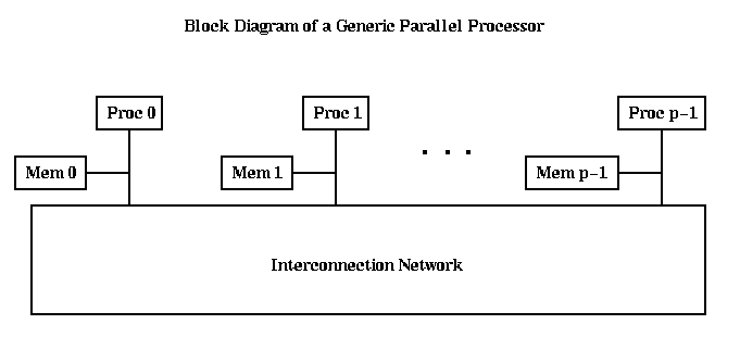
Second, we distinguished betweenThe block diagrams below are quite schematic, and do not reflect the actual physical structure an any particular machine. Nonetheless, they are quite useful for understanding how these machines work. For more detailed block diagrams, see the lectures in CS 258, or click here.
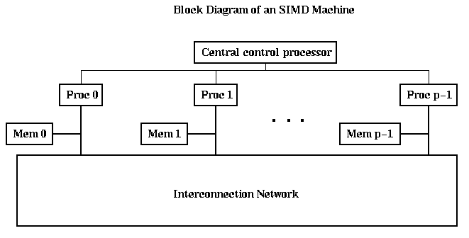
A simple block diagram of an SIMD machine is shown below. The central control processor sends instructions to all the processors along the thin lines, which are executed in lock step by all the processors. In other words, the program resides in the central control processor, and sent to the individual processors one instruction at a time. This block diagram describes the Maspar and CM-2.
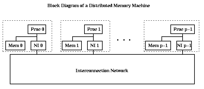
A simple block diagram of a distributed memory MIMD machine is shown below. Each processor node (shown enclosed by dotted lines) consists of a processor, some local memory, and a network interface chip (NI), all sitting on a bus. Loads and stores executed by the processor are serviced by the local memory in the usual way. In addition, the processor can send instruction to the NI telling it to communicate with an NI on another processor node. The NI can be a simple processor which must be controlled in detail by the main processor (as on the Paragon can be viewed this way). This class also includes the IBM SP-2 and NOW (network of workstations).
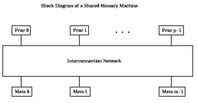
A simple block diagram of a shared memory MIMD machine is shown below. This particular diagram corresponds to a machine like the Cray C90 or T90, without caches, and where all it takes equally long for any processor to reach any memory location. There is a single address space, with each memory owning 1/m-th of it. (There need not be as many memories as processors.) Typically, the memory is interleaved, which means that address i is actually located in Memory i mod m, at offset floor(i/m); this assumes m is a power of 2.
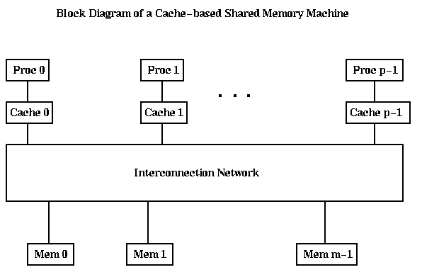
A simple block diagram of a cache based shared memory MIMD machine like the SGI Power Challenge is shown below. Here, each processor has a cache memory associated with it. The tricky part of designing such a machine is to deal with the following situation: Suppose processors i and j both read word k from the memory. Then work k will be fetched and stored in both Mem i and Mem j. Now suppose Proc i writes work k. How will Proc j find out that this happened, and get the updated value? Making sure all the caches are updated this way is called maintaining cache coherency; without it, all processors could have inconsistent views of the values of supposedly identical variables. There are many mechanisms for doing this. One of the simplest is called snoopy caching, where the interconnetion network is simply a bus to which all caches can listen simultaneously. Whenever an address is written, the address and the new value are put on the bus, and each cache updates its own value in case it also has a copy.
The Cray T3D, also falls into this category, since it has a global shared memory with caches, but it operates differently. There are m=p memories, and they are closely attached to their respective processors, rather than all being across the interconnection network. Referring to nonlocal memory requires assembling a global address out of two parts, in a segmented fashion. Only local memory is cachable, so cache coherence is not an issue.
For more detailed blocks diagrams of some of these architectures
Here is the sort of algorithm one can write on this perfect parallel computer. It uses n^2 processors to sort n distinct numbers x(1),...,x(n) in constant time, storing the sorted data in y:
    for all ( i=1,n, j=1,n )  if ( x(i) > x(j) ) then count(i) = 1
    for all ( i=1,n ) y(count(i)+1) = x(i)
The algorithm works because count(i) equals the number of data items
less than x(i). This algorithm is too good to be true, because the
the computer is too good to be built: it assume n^2 processors
are available, and that all can access a single location at a time.
Even the less powerful
EREW PRAM (Exclusive Read Exclusive Write PRAM) model, where at
most one processor can read or write a location at a time (the
others must time in turn), does not capture the characteristics of
real systems. This is because the EREW PRAM model ignores the capacity
of the network, or the total number of messages it can send at a time.
Sending more messages than the capacity permits leads to contention,
or traffic jams, for example when all processors
try to reach different words in the same memory unit.
At this point we have two alternatives. We can use a detailed, architecture specific model of communication cost. This has the advantage of modeling accuracy, and may lead to very efficient algorithms highly tuned for a particular architecture. However, it will likely be complicated to analyze and need to change for each architecture. For example, later we will show how to tune matrix multiplication to go as fast as possible on the CM-2. This algorithm required clever combinatorics to figure out, and the authors are justifiably proud of it, but it is unreasonable to expect every programmer to solve a clever combinatorics problem for every algorithm on every machine.
So instead of detailed architectural models, we will mostly use an architecture-independent model which nonetheless captures the features of most modern communication networks. In particular, it attempts to hide enough details to make parallel programming a tractable problem (unlike many detailed architectural models) but not so many details that the programmer is encourage to write inefficient programs (like the PRAM).
This "compromise" model is called LogP. LogP has four parameters, all measured as multiples of the time it takes to perform one arithmetic operation:
Furthermore, it assumed that the network has a finite capacity, so that at most L/g message can be in transit from any processor to any processor at any given time. If a processor attempts to send a message that would exceed this limit, it stalls until the message can be sent without exceeding the capacity limit.We will often simplify LogP by assuming that the capacity is not exceeded, and that large messages of n packets are sent at once. The time line below is for sending n packets. This mimics the "store" in Split-C, because there is no idle time or acknowledgement sent back, as there would be in blocking send-receive, for instance. oS refers to the overhead on the sending processor, gS the gap on the sending processor, and oR the overhead on the receiving processor.
-----------> Time

| oS |   L   | oR |          packet 1 arrives
|  gS  | oS |   L   | oR |          packet 2 arrives
       |  gS  | oS |   L   | oR |          packet 3 arrives
              |  gS  | oS |   L   | oR |          packet 4 arrives
                         ...
                     |  gS  | oS |   L   | oR |          packet n arrives
By examining this time line, one can see that the total time to send
n message packets is
2*o+L + (n-1)*g = (2*o+L-g) + n*g = alpha + n * beta
Some authors refer to alpha = 2*o+L-g as the latency instead of L, since
they both measure the startup time to send a message. The following
table gives alpha and beta for various machines,
where the message packet is taken to be 8 bytes.
Alpha and beta are normalized so that the time for one flop
done during double precision (8 byte) matrix multiplication is
equal to 1. The speed of matrix multiplication in Mflops is also
given.
      Machine        alpha   beta   Matmul Mflops      Software

     Alpha+Ether      38000   960       150          assumes PVM
     Alpha+FDDI       38000   213       150          assumes PVM
     Alpha+ATM1       38000    62       150          assumes PVM
     Alpha+ATM2       38000    15       150          assumes PVM
     HPAM+FDDI          300    13        20
     CM5                450     4         3          CMMD
     CM5                 96     4         3          Active Messages
     CM5+VU           14000   103        90          CMMD
     iPSC/860          5486    74        26
     Delta             4650    87        31
     Paragon           7800     9        39
     SP1              28000    50        40
     T3D              27000     9       150          Large messages(BLT)
     T3D                100     9       150          read/write
(Comments on the table: Most data is measured, some is estimated. Most are for blocking send/receive unless otherwise noted. Details to be filled in!)
The most important fact about this table is that alpha>>1 and beta>>1. In other words, the time to communicate is hundreds to thousands of times as long as the time to do floating point operations. This means that an algorithm that does more local computation and less communication is strongly favored over one that communicates more. Indeed, an algorithm that does fewer than a hundred floating point operations per word sent is almost certain to be very inefficient.
The second most important fact about this table is that alpha >> beta, so a few large messages are much better than many small messages.
Because of these two facts, alpha and beta tell us much about how to program a particular parallel machine, by telling us how fast our programs will run. If two machines have the same alpha and beta, you will probably want to consider using similar algorithms on them (this also depends on whether they are both MIMD or both SIMD, both shared memory or both distributed memory too, of course).
The fact that different machines in the table above have such different alpha and beta makes it hard to write a single, best parallel program for a particular problem. For example, suppose we want to write a library routine to automatically load balance a collection of independent tasks among processors. To do this well, one should parameterize the algorithm in terms of alpha and beta, so it adjusts itself to the machine. We will discuss such algorithms later.
Let us discuss the above table in more detail. The first 4 lines give time for a network of DEC Alphas on a variety of local area networks, ranging from 1.25Mbyte/sec ethernet to 80MByte/sec ATM. Alpha remains constant in the first 4 lines because we assume the same slow message passing software, PVM, which requires a large amount of time interacting the OS kernel. Part of the NOW project is to improve the hardware and software supporting message passing to make alpha much smaller. A preliminary result is shown for the HPAM+FDDI (HP with Active Messages).
There are three lines for the CM-5, because the CM-5 comes both with and without vectors units (floating point accelerators), and because it can run different messaging software (CMMD and AM, or Active Messages).
The next three lines are a sequence of machine built by Intel. The IBM SP-1 consists of RS6000/370 processors; the IBM SP-2 uses RS6000/590 processors. The T3D is built by Cray, and consists of DEC Alphas with network and memory management done by Cray.
The messaging software can often introduce delays much larger than that of the underlying hardware. So be aware that when you or anyone else measures performance on a machine, you need to know exactly which message software was used, in order to interpret the results and compare them meaningfully with others. For example, PVM is slow both because it does all its message sending using UNIX sockets, which are slow, and also because it has a lot of error checking, can change data formats on the fly if processors with different formats are communicating, etc.
The basic tradeoff in designing the interprocessor communication network is between speed of communication and cost: high speed requires lots of connectivity or "wires", and low cost requires few wires. In this section we examine several designs for the network, and evaluate their costs and speeds. We will also see to what extent the LogP model can depart from reality.
The network typically consist not just of wires but routing processors, which may be small, simple processors or as powerful as the main processors (eg. the Intel Paragon uses i860 processors for both). Early machines did not have routing processors, so that a single processor had to handle both computation and communication. Newer machines use separate routing processors so communication and computation can proceed in parallel.
Networks always permit each processor to send a message to any other processor (one-to-one communication). Sometimes they support other more complicated collective communications like broadcast (one-to-all), reduction and scan. We will first consider one-to-one communication.
We will classify networks using the following criteria.
This classification is coarse, and many networks are hybrids with features from several categories.For each network, we will give its
LogP and the alpha+n*beta communication cost model ignore diameter because they ignore the fact that messages to nearest neighbors may take less time than messages to distant processors, by using average values for alpha and beta. This reflects the fact that on modern architectures most of the delays are in software overhead at the source and destination, and relatively little in latency in between. In particular, this means that we often can ignore topology in algorithm design.
LogP incorporates bisection width indirectly by limiting the capacity of the network.
Bus. This is the simplest and cheapest dynamic network. All processors sit on a shared bus (wire), which may be written to by at most one processor at a time. This is the way the CPU, memory, and perhaps I/O devices are connected internally in a processor. The diameter is 1, since every processor is directly connected to every other processor. The bisection width is also 1, since only one message may be sent at a time. This is also the way a network of workstations is connected, if there is just one physical medium, like an Ethernet. More sophisticated networks, like ATMs, consist of busses connected with small crossbars.
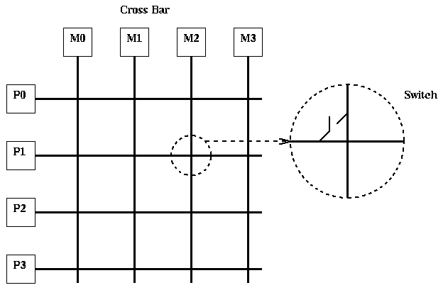
Crossbar (or Xbar). This is the most expensive dynamic network, with each processor directly connected to every other processor. It is used in mainframes, and smaller ones appear as components in hybrid networks. There are p^2 switches connecting every processor to every other processor, and at most p may be connected at a time, forming a permutation. The diameter is 1, and the bisection with is p/2, since any p/2 processors can always communicate with the other p/2 processors.
Perfect Shuffle and Omega Network.. A perfect shuffle connects p = 2^m (routing) processors to another p (routing processors) as follows. All processors have a unique m-bit binary address. A perfect shuffle connects the processor with address s with the processor with address cshiftl(s) = circular-shift-left of s by 1 bit. For example if there are 8=2^3 processors, processor s1s2s3 is connected to processor s2s3s1 (see the figure below). An omega network consists of m perfect shuffles connected end to end, with a switch connecting adjacent pairs of wires between each perfect shuffle. Switch i can either send a message "straight across", if bit i of the source processor number equals bit i of the destination processor number, or send it to the adjacent wire if the two bits differ (see the figure). The omega network routs a message dynamically from source processor to destination processor as follows. Assume for simplicity that there are 8 processor, so the source has address s1s2s3, and the destination has address d1d2d3.
   Initial (source) location:     s1s2s3
   Location after first shuffle:  s2s3s1
   Location after first switch:   s2s3d1  (straight across if s1 = d1,
                                           adjacent wire if s1 != d1)
   Location after second shuffle: s3d1s2
   Location after second switch:  s3d1d2  (straight across if s2 = d2,
                                           adjacent wire if s2 != d2)
   Location after third shuffle:  d1d2s3
   Location after third switch:   d1d2d3  (straight across if s3 = d3,
                                           adjacent wire if s3 != d3)
   Final (destination) location:  d1d2d3
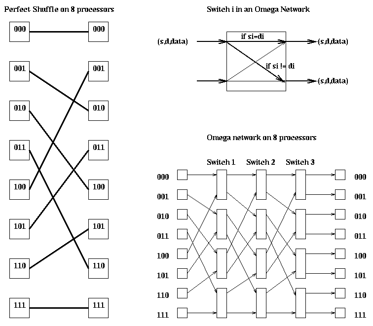
The diameter is m=log_2 p, since all message must traverse m stages. The bisection width is p. This network was used in the IBM RP3, BBN Butterfly, and NYU Ultracomputer.