CS 184: COMPUTER GRAPHICS

|
PROBLEM # 1:
How would you construct a reasonable scene hierarchy for the scene on the left?
PROBLEM # 2:
Assume a scene has a bright red triangle in it.
Try to list all the reasons why the display of that scene might NOT show any bright red pixels.
|
PREVIOUS
< - - - - > CS
184 HOME < - - - - > CURRENT
< - - - - > NEXT
Lecture #6 -- Mon 2/7/2011.
Crucial Concepts from Last Lecture:
Complex scenes are described using hierarchically nested groups of objects (and of other groups) with relative transformations.
Entities that transform together should be grouped together.
An object or group of objects can be instantiated multiple times -- in different places, with different orientations, and different scales.
Different properties get inherited differently down the hierarchy.
The conceptual scene structure is expressed in a corresponding scene graph, which can also be captured in a scene description file:
(G group_A
(I inst_1 geom (Xform A) (Xform B) (Xform
C) ) ## should result in: [Xform C] * [Xform B] * [Xform A] * [geom]
(I inst_2 bird (S
1.1 1.6 ) (T 5 3.4 )
(color 1 0.8
0.2 ) ) ## stretched, orange bird;
(I inst_3 flock (S 0.8
0.8 ) (T {t*0.2} {4+t*0.1}) ) ##
shrunk, uncolored flock of birds, moving to the right and up;
(I inst_4 UFO (R
{t*20} ) (T 8 9 ) (color {sin(t*45*dgr)}
{cos(t*66*dgr)} 0.2 ) ) ## UFO,
rotating 20 degrees per frame around its center, and changing color.
)
Here is an example of a hierarchical scene: 18-Wheeler and a discussion how its hierarchy needs to get modified when there is a flat tire.
Rendering: Getting parts of such a scene onto a diplay
Rendering Principles: Comparison of Physical Camera, Clasical Rendering Set-up, and Ray-Casting
In physical rendering (photography), photons reflected off the surface elements of the scene get captured by the lens and focussed onto film.
In a Classical CG Rendering Pipeline the scene graph will be traversed and expanded (flattened) into a full scene tree,
and every leaf will be properly transformed and projected onto the image plane.
In Ray-casting: For each pixel on the display screen, shoot a ray
from the eye into the scene and determine what it hits, and what color
we should put there.
The apparant color of a particular spot in the scene depends on its
surface properties, on what light illuminates it, and how the re-emitted
light is transformed on the way to the eye/camera.
That is what we focus on in Assignment#4. Schematic of the ray-tracer program.
We will use just a few spheres, so it is easy to determine what any ray hits;
-- but spheres can look quite different depending on surface properties and lighting conditions.
Color, Lighting, Shading
CLARIFICATION OF TERMS:
Color is represented with 3 components: RED, GREEN, BLUE,
or (RGB) for short.
Almost all CG systems work with a 3-vector color basis.
This works because the human visual system has three types of
color receptors (more later in the semester).
A surface color, is characterized by the additive mixture of RGB colors that get
reflected when the surface is illuminated with white light ( R=1; G=1;
B=1 ).
Illumination (lighting) models:
tell us what brightness and what color to expect (physically) on each
surface.
Shading / rendering:
concerns (efficient) techniques to produce the apparent brightness values on the
display.
For instance: To give the appearance of smooth and smoothly colored
objects,
we may calculate each pixel color as a weighted blend of the colors
of nearby vertices.
For simplicity (and assuming that the color differences are not
too large),
we interpolate the three RGB components separately.
In the context of scan-line based rasterization,
(to be discussed soon),
we simply do a linear interpolation along the polyhedron edges,
and a linear interpolation across a face from the left edge to right
edge along the current scan line.
This bi-linear interpolation of color (and brightness) differs
somewhat from the
interpolation of z-depth -- which we assumed to be a planar
function.
The shading/illumination function is NOT typically planar !
(More on that later).
But first we need to learn how to determine the intensities (colors) at arbitrary points
of an object.
For that we need an illumination / lighting model.
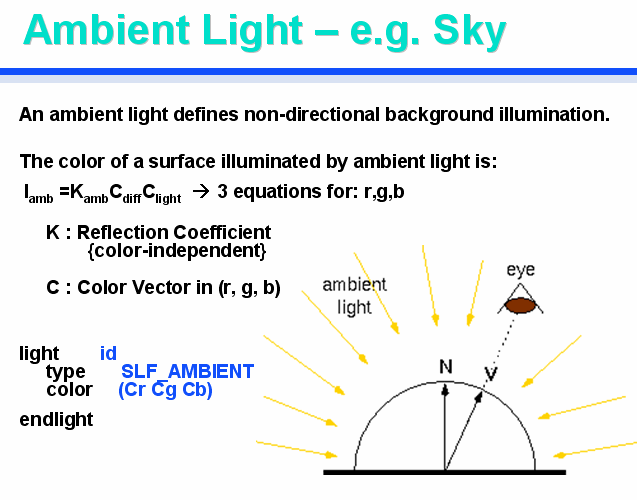
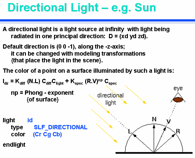
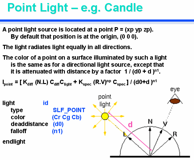
Lights and Illumination
Definition of important
directions and unit vectors: L, V, N, R, H.
Preview of all the coefficients that you will see shortly: C's and
K's
Types of Light Sources: Light source models and their key parameters (SLIDE notation)
Ambient Light (e.g., sky): Iamb, Clight (r,g,b).
Directional Light (e.g., sun): Idir, Clight (r,g,b). -- Calculate: L.
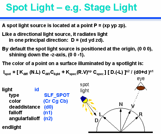
Point Light (e.g., candle): Ipoint, Clight (r,g,b), d0, n1. -- Calculate: L, d.
Spot Light (e.g., stage light): Ispot, Clight (r,g,b), d0, n1, n2. -- Calculate: L, D, d.
Superposition Law: Calculate the effects of each light individually and sum all the resulting
effects.
(I.e., there is no interaction between photons).
Lighting /(Surface) Models
Illumination (Lighting / Surface) models:
They tell us what brightness and what color to expect
(physically) at a surface point.
1. Lambert Surfaces
This is an idealization of diffusely reflecting (chalky)
surfaces.
Their main advantage is that the apparent brightness of any
spot on the surface is viewer-independent.
LAMBERT SURFACES -- what we see:
Formula that shows view-angle independence.
LAMBERT PHYSICS -- why that is so:
Show where the cosine factors are coming from and why they cancel:
Light absorption falls off with the cosine of the angle between
light and face normal.
This is because a surface at a non-perpendicular angle in a flux of
photons captures fewer
photons (by a cos- factor), since it exposes a smaller cross sectional
area to the photon stream.
This effect is viewer independent and can be pre-calculated once at
scene construction time.
All the lighting energy that hits the surface gets absorbed temporarily,
then some percentage gets reemitted.
The percentage of light re-emitted in a particular direction
depends on the properties of the surface, e.g., Kd, Cd
{R,G,B};
For Lambertian (chalky) surfaces the re-emission probability has broad distribution
which has a maximum perpendicular to surface; it falls off with the cos of the angle away from the normal. The reason
is that grazing photons
have a hard time escaping the "rugged" chalky surface, i.e., they get trapped
again by protrusions.
Emission probability:  and Slanted viewing situation:
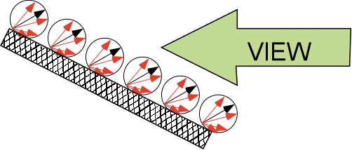
When viewing a surface from an arbitrary angle, this fall-off
is compensated by the fact that,
as we see the surface more foreshortened, we also crowd more emission
centers into
the apparent solid angle of our viewing field by 1/cos . ( DEMO
with black page with white dots.)
Thus a chalky Lambert surface has an apparent brightness
that does not vary with view direction.
Flat polygons will appear of uniform brightness when uniformly lit,
and they all keep a constant brightness from all view points!
Thus the output spans for a flat polygon can be of uniform brightness
from left to right edge (even under close-up, wide-angle viewing!).
Note: Our sun is also a "Lambert type emitter" -- Thus its apparent intensity is constant
across the whole perceived "flat disk".
When do chalky spheres appear as uniformly shaded (apparently flat) disks ?
When do they appear as depth modulated 3D objects with varying brightness ?
2. Perfect Mirrors
Shiny surface with complete specular reflection.
Reflection laws: L, N, R in same plane; incident angle = reflection
angle (against normal),
but R is on the other side of the normal vector.
The result is, that we see a bright reflection spot where
the camera lies in the R direction;
everywhere else the surface is dark !
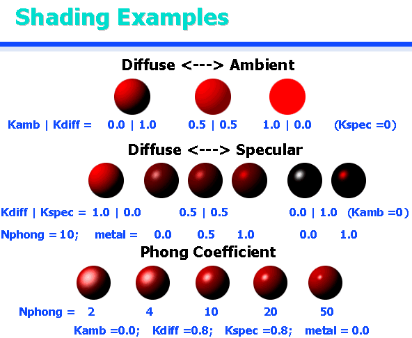
3. Phong Approximation of Real Surfaces
Real surfaces are a mixture of chalky properties and of a dull, dusty mirror.
They have some diffuse as well as some specular reflection.
==>
The reflected beam is spread out in a small angle around the unit vector
R.
Phong model: Models the reflective component on a real surface
as a "fuzzy club" shape around R
Its intensity falls of with a user definable power of the cosine of
the deviation angle from the ideal R direction.
Phong Illumination/Lighting/Surface Model:
Show effect of exponent of cosine function.
Phong Highlight on flat glossy surface:
Even uniform directional light falling on a flat surface can produce
non-uniform brightness,
if surface is partially reflective and we use a Phong illumination
model.
4. Advanced Approximations of Real Surfaces: ... [ NEXT LECTURE ]
Reading Assignments:
Study: ( i.e., try to understand fully, so that you can answer
questions
on an exam):
Shirley 2nd Ed. [ 9.1-9.2;
10.1-10.4 ]. Shirley 3rd Ed. [ 4.1-4.6; 10.1-10.2 ].
Lecture notes (your own, and the ones on-line)!
Feb. 14: Take-Home Exam (open book): Due Feb.16. ==> Reserve 2-3 hrs of quiet time!
Programming Assignments:
Assignment #3 is due (electronically submitted) before Friday 2/11, 11:00pm. <== THIS ASSIGNMENT CAN BE DONE IN PAIRS !
(A#4: Basics of ray-tracing, will be done individually again)
PREVIOUS
< - - - - > CS
184 HOME < - - - - > CURRENT
< - - - - > NEXT
Page Editor: Carlo
H. Séquin