CS 184: COMPUTER GRAPHICS
PREVIOUS
< - - - - > CS
184 HOME < - - - - > CURRENT
< - - - - > NEXT
Lecture #25 -- Mon 4/25/2011.
Question of the Day:
Two paintings look exactly the same when illuminated with bright sun light.
Will they still look the same when viewed through sun glasses?
Will they still look the same when viewed under artificial lights?
What is the basis for your conlcusions?
Color Spaces
There are many useful color spaces based on physics, the
human eye, the needs of computer graphics, the way artists' mix paints
...
Color Wheels (Rainbow colors wrapped around a circle)
Artists use: Red, Yellow, Blue.
==> Subtractive mixing (filters, paint mixing).
For color printers we now use:
Cyan, Yellow, Magenta, and a good Black ==> CYMK system
Computer Scientist’s wheel: Red, Green, Blue. ==> Additive mixing
(light beams; CRT).
We are missing some colors: Where is: brown, olive, pink, dark blue ...
?
Color space is 3-dimensional to accommodate also brightness and saturation
variations in addition to hue:
Graphics hardware view: RGB cube, store 3 intensity values for
display on CRT.
Extension of the additive color wheel to a cone (6-sided pyramid or cone)
==> HSV.
Alternative: HLS: Double hex-cone. White/black at tips;
saturated colors on rim at height 0.5.
Physicist’s View: continuous spectrum, infinite dimensions!
Typical spectrum has some broad bumps plus some sharp spectral lines
(added or subtracted). Example: Quasar-Spectrum
... So why can computer graphics get away with only three colors (R G B)?
The human visual system has three types of cones.
It can only take three wavelength-samples,
each over relatively broad color bands.
Sensitivity of these cones differs: green most sensitive, blue least sensitive.
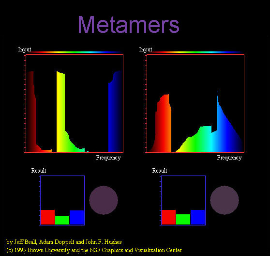
Metamers: Colors that look the same (P), but have different spectra (L1,
L2).
Comparative measurements are done with a color-matching set-up:
 The two principal set-ups.
3 superposed lights (A,B,C) are compared with test color (T).
You can match almost all colors, as far as human perception
goes with an additive mix of the 3 base colors.
The remainder can be matched when one of the 3 colors is placed on
the test light -- to produce a subtractive effect.
This results in color matching functions with positive and negative
coefficients.
==> Perceptual
space is 3-dimensional. (1st Grassman Law )
Grassman’s Laws (of color mixing):
(Grassman measured RGB coordinates of all perceptual colors in 5nm steps through visual spectrum,
in 1931)
Law #1. Perceptual space is 3-dimensional.
(see above) A basis of three primary colors is sufficent to generate all colors visble to humans.
Law #2. Metamer mix (add) to yield metamers:
L1, L1’ ==> P1; L2, L2’ ==> P2; then for any a, b :
a*L1 + b*L2 ==> P3; then a*L1’ + b*L2’ ==> P3.
(This is not true for paints or pigments with non-additive behavior; see example
with filter (dashed) below).
Here filter makes no difference -- but here it reduces intensity dramatically!
Law #3. As physical color is varied continuously, perceptual color also
varies continuously.
(Continuity of the perceptual process).
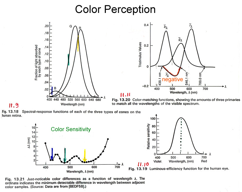
The human retina has three kinds of color sensors (i.e., cones) with peak sensitivities
near 440nm (blue), 545nm (yellow-green), and 580nm (orange) in the
visual part of the spectrum.
The blue sensor is much less responsive than the other two (Foley Fig.13.18).
(There are also "rods" that are more sensitive, but are essentially
black&white sensors).
This leads to the tri-stimulus theory of color perception: which
postulates that colors can be synthesized
from weighted sums of some primary colors, typically in the red, green,
and blue range.
However this is not possible with only positive weighting factors;
some blue-green components of the spectrum require a negatively weighted
red component (Foley Fig.13.20).
This means that the desired color sample has to be changed (de-saturated) with
some red light,
so that it can then be matched by positive blue and green components.
Frequency sensitivity of the eye varies from about 2nm for yellow and
blue to about 10nm near the edge of the visible spectrum.
Overall, about 128 fully saturated hues can be distinguished.
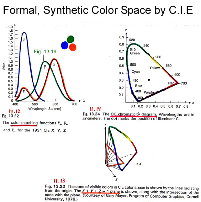
A perceptual
color space was formally defined in 1931 by the Commission International
de l’Eclairage (CIE).
To avoid the need for negative weights, they defined a new set of basis
vectors (primary colors) X, Y, Z,
that lie completely outside the range of all visible RGB values,
so that the color matching functions x(l),
y(l), z(l) for any
visible hue become entirely positive (Foley Fig.13.22).
In addition, the y(l) function is
defined so that it matches the luminosity-efficiency of the human eye (Foley
Fig.13.19);
thus it can be used by itself as an intensity channel.
The transformation from the original RGB color matching functions to
the CIE color matching functions is linear.
If we intersect the visible portion of the CIE color space with a plane
X+Y+Z=1 (about equal brightness),
then we get the horseshoe-shaped region depicted in the CIE
chromaticity diagram.
The fully saturated, pure, spectral colors all lie on the curved part
of the horseshoe.
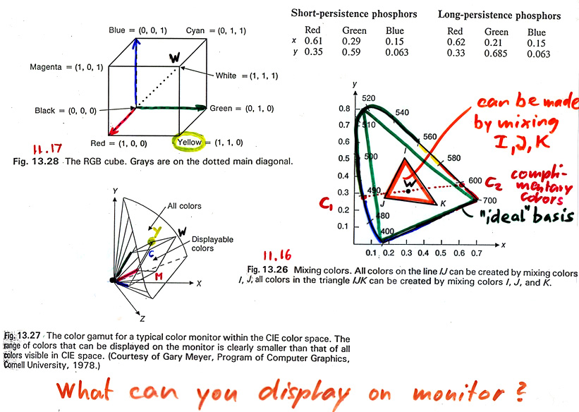
Somewhere near the center is a point defined as "white".
Colors lying opposite this "white" point are called complementary
colors (Foley Fig.13.26).
A particular tri-stimulus
(3-color) display system has three primaries: I,J,K (Foley Fig.13.27).
It can display only the colors that lie within its convex hull
(=triangle).
(Can only use linear combinations of the 3 base colors
with coefficients [0,1]).
Thus we would like to make this triangle as large as possible (==> "ideal
basis"),
but we are limited by what colors of phosphor (or LED's, or gas-discharge)
are available.
The typical CRT display can cover less than half of the visible domain
of colors!
Typical Exam Question:
3D
Color Spaces
Learning by Doing:
Additive
Mixing
Subtractive
Mixing
Metamers
Color
Mixing/Filtering Combination
and
many more ...
Transparency
Transparency measures what fraction of light passes through
a surface or body;
that fraction is indicated by the transmission coefficient kt.
Opacity (a) indicates what fraction
is held back; a=1 means: completely opaque.
By definition: kt+a=1
Translucency is a partly transparent object in which the scattering effect dominates; example: frosted glass.
There are many ways to implement partially transparent/opaque objects:
Any of the Photon-, Path-, Cone-, Beam-tracing methods discussed
are a natural way to deal with a (partially) transparent object T;
for instance:
At the surface of object T, we split the ray into a primary ray that
returns the color of object T with some weighted percentage,
and into a secondary ray that passes through the medium and returns
information "from behind" with the complementary percentage.
This information could be further attenuated or discolored, depending
on the thickness of the body T.
OpenGl offers another mechanism: alpha blending.
A fourth channel a is established
-- in addition to R, G, B.
Thus for each surface, vertex, or pixel we can define four values:
(RGBa).
If a-blending is enabled, the fourth parameter a
determines
how the the RGB values are written into the frame buffer:
typically the result is a linear combination (or blend) of the
contents already in memory and the new information being added.
Filtered Transparency:
Assume that in the frame buffer there is a pixel (Fr, Fg, Fb, Fa),
and we want to place a new pixel with opacity a
in front of it (Nr, Ng, Nb, Na):
We can achieve the desired result with: ( a*Nr
+ kt*Fr, a*Ng
+ kt*Fg, a*Nb
+ kt*Fb, a*Nar
+ kt*Fa );
this corrsponds to placing a filter of opacity a
in front of an already rendered scene.
(if a=1 the New pixel dominates).
For this blending function to work, the transparent polygons have to
be rendered after (in front of) the opaque objects.
For multiple filter polygons, the effect is calculated recursively
back-to-front.
Interpolated Transparency:
In a different situation, we might want to form a composite image from
m
candidate images (e.g. in Image-based Rendering);
In this case, the compositing function might look like: ( sum(Nri)/m,
sum(Ngi)/m, sum(Nbi)/m,
sum(Nai)/m, )
OpenGL provides many different blending functions to take care of many
commonly occuring situations.
Interpolated transparency can be realized by rendering only a subset of
the pixels associated with the image of the transparent object;
in the other pixels, the object behind the "screen-door" object is
rendered.
(the low-order bits in the pixel address determine to which subset
a pixel belongs.)
This technique is limited to a very small number of overlapping transparent
media,
and it can produce some undesirable Moire effects.
(==> Sampling problems! ==> next lecture).
HKN Survey
Reading Assignments:
Shirley: 2nd Ed: Ch.19.1 - 19.2; Ch.20
3rd Ed: Ch.20.1 - 20.2; Ch.21
CS 184 Course Project: Consult Project Page!
As#12 = PHASE_3:
Intermediate Progress report: Show evidence of the basic core of your project working.
(more details will be forthcoming).
Due Monday May 2, 11pm (worth another 15% of project grade).
PREVIOUS
< - - - - > CS
184 HOME < - - - - > CURRENT
< - - - - > NEXT
Page Editor: Carlo
H. Séquin