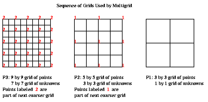
This idea of using a coarse approximation of a problem to approximate its solution, (and recursively using a yet coarser approximation of the coarse problem) is used in a variety of fast algorithms; we will see it again when we discuss graph partitioning.
The second way Multigrid uses divide-and-conquer is in the frequency domain. This requires us to think of the error as a sum of sine-curves of difference frequencies. Then the work we do on a particular grid will eliminate the error in half of the frequency components not eliminated on other grids. In particular, the work performed on a particular grid -- averaging the solution at each grid point with its neighbors, a variation of Jacobi -- makes the solution smoother, which is equivalent to getting rid of the high frequency error. We will illustrate these notions further below.
For a more detailed mathematical introduction to the multigrid algorithm, see "A Multigrid Tutorial" by W. Briggs, SIAM, 1987. For a matlab implementation of multigrid click here.
We begin by stating the algorithm at a high level, and then fill in details. It turns out to be convenient to consider an (2^m-1)-by-(2^m-1) grid of unknowns, rather than the 2^m-by-2^m grid favored by the FFT. We add the nodes at the boundary, which have the given value 0, to get a (2^m+1)-by-(2^m+1) grid on which the algorithm will operate. We let n=2^m+1. These grids are shown below.
We let P(i) denote the problem of solving a discrete Poisson equation on a (2^i+1)-by-(2^i+1) grid, with (2^i-1)^2 unknowns. The problem is specified by the grid size i, the coefficient matrix T(i), and the right hand side b(i). We will generate a sequence of related problems P(m), P(m-1), P(m-2), ... , P(1) on coarser and coarser grids, where the solution to P(i-1) is a good approximation to the solution of P(i).

We will let b(i) be the right-hand-side of the linear system P(i). We will let x(i) denote an approximate solution to P(i). Thus, x(i) and b(i) are (2^i-1)-by-(2^i-1) arrays of values at each grid point. To explain how the algorithm works, we need some operators which take a problem on one grid, and either improve it or transform it to a related problem on another grid:
( b(i-1), x(i-1) ) = R(i)( b(i), x(i) )
We will see that restriction is implemented simply
by computing a weighted average of each grid point value with its nearest
neighbors.
( b(i), x(i) ) = In(i-1)( b(i-1), x(i-1) )
Its implementation also requires just a weighted average with nearest
neighbors.
x_improved(i) = S(i)( b(i), x(i) )
The improvement is to damp
the "high frequency components" of the error. We will explain what this
means below. It is also implemented by averaging with nearest neighbors,
and is a variation of Jacobi's method.
This is enough to state the basic algorithm, the Multigrid V-cycle (MGV).
  function MGV( b(i), x(i) )       ... return an improved
                                   ... solution x(i) to P(i)
    if i = 1                       ... only one unknown
       compute the exact solution x(1) of P(1)
       return ( b(1), x(1) )
    else
       x(i) = S(i)( b(i), x(i) )  ... improve the solution
       ( b(i), d(i) ) = In(i-1)( MGV( R(i)( b(i), x(i) ) ) )
                                  ... solve recursively
       x(i) = x(i) - d(i)         ... correct fine grid solution
       x(i) = S(i)( b(i), x(i) )  ... improve solution some more
       return ( b(i), x(i) )
    endif
In words, the algorithm does the following:
R(i)( b(i), x(i) ).
MGV( R(i)( b(i), x(i) ) ).
In(i-1)( MGV( R(i)( b(i), x(i) ) ) ).
x(i) = x(i) - d(i)
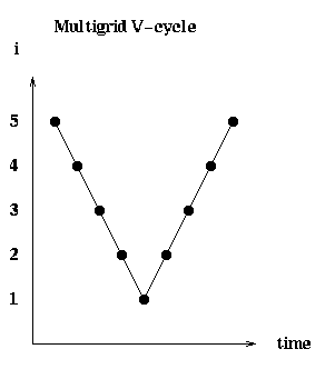
We now know enough to get a big-Oh complexity analysis for the algorithm. On a serial machine, the work at each point in the algorithm is proportional to the number of unknowns, since the value at each grid point is just averaged with its nearest neighbors. Thus, each point at grid level i on the "V" in the V-cycle will cost (2^i-1)^2 = O(4^i) operations. If the finest grid is at level m, the total serial work will be given by the geometric sum
sum_{i=1}^m O( 4^i ) = O( 4^m ) = O( # unknowns )
So the total serial work is proportional to the number of unknowns.
On a PRAM, we could compute all the nearest neighbor averages required at each grid point in unit time, with one processor per grid point. Thus, the time required on a PRAM is just proportional to the number of dots on the V in the V-cycle, namely O(m) = O( log #unknowns ).
The ultimate Multigrid algorithm uses the Multigrid V-cycle just described as a building block. It is called Full Multigrid (FMG):
   function FMG( b(m), x(m) )
     compute the exact solution x(1) of P(1)
     for i= 2 to m
         ( b(i), x(i) ) = MGV( In(i-1)( b(i-1), x(i-1) ) )
     end for
In words, the algorithm does the following:
In(i-1)( b(i-1), x(i-1) ).
MGV( In(i-1)( b(i-1), x(i-1) ) )
Now we can do the overall Big-Oh complexity analysis. The picture in (grid number i, time) space is:
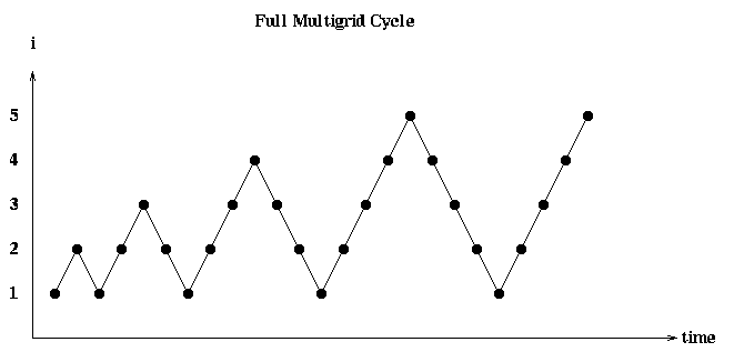
There is one V in this picture for each call to MGV in the inner loop of FMG. On a serial machine, the V starting at level i costs O(4^i), as before. Thus the total serial cost is given by the geometric sum.
sum_{i=1}^m O( 4^i ) = O( 4^m ) = O( # unknowns )
The cost on a PRAM is also the sum of the costs of each V:
sum_{i=1}^m O( i ) = O( m^2 ) = O( (log # unknowns)^2 )
This completes the serial and PRAM complexity analyses of Multigrid:
the serial complexity is optimal, in the sense that a constant amount
of work per unknown is performed. The PRAM complexity is the square
of the optimal (which was attained by the FFT), namely
O( log( # unknowns )^2 ) instead of
O( log( # unknowns ) ). After explaining the operators R(i-1), In(i) and S(i)
in more detail, we will do a more complete complexity analysis taking
communication into account.
To make the exposition and figures simpler, we will use 1D problems to explain the details of the algorithm. Thus, P(i), as shown below, will be a problem on a 1D grid of 2^i+1 points, with the middle 2^i-1 being the unknowns.

We will let T(i) be the coefficient matrix of problem P(i), that is a scaled (2^i-1)-by-(2^i-1) tridiagonal matrix with 2s on the diagonal and -1s on the off-diagonal. The scale factor 4^(-i) is the 1/h^2 term that shows up because T(i) is approximating a second derivative on a grid with grid spacing h=2^(-i).
                     [  2  -1                 ]
                     [ -1   2  -1             ]
     T(i) = 4^(-i) * [     -1   2  -1         ]
                     [       ... ... ...      ]
                     [             -1  2  -1  ]
                     [                -1   2  ]
To understand why Multigrid works so well, we need to think of the
solution vector, and the error in the solution, as linear combinations of
certain basis vectors, which are essentially sine-curves of different
frequencies, the way one does in Fourier analysis. This same idea underlay
the use of the FFT in solving this problem. As with the FFT, these sine-curves
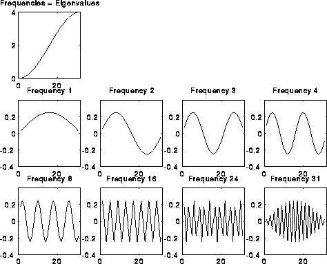
are in fact the eigenvectors of the T(i) matrix above. The following
figure shows some of these sine-curves when i=5, so T(5) is 31-by-31.
The top plot is a plot of the eigenvalues (frequencies) of 4^5*T(5), from
lowest to highest. The subsequent plots are the eigenvectors (sine-curves),
starting with the lowest 4 frequencies, and then a few more frequencies up
to the highest (number 31).
If we let v(j) be the j-th eigenvector of T(i), and V the eigenvector matrix V=[v(1),v(2),...] whose j-th column is v(j), then as described before V is an orthogonal matrix. Any vector x can be written as a linear combination of the v(j). Here is how:
x = sum_{j=1}^{2^i-1} alpha(j)*v(j) = V*alpha
where alpha = [alpha(1), alpha(2), ...]' is a column vector of
coefficients. Writing
x = I*x = (V*V')*x = V*(V'*x) = V*alpha
we see that alpha(j) = v(j)'*x.
We call alpha(j) the j-th frequency component of x, ranging from
alpha(1) (the lowest frequency component) to alpha(2^i-1) (the highest
frequency component).
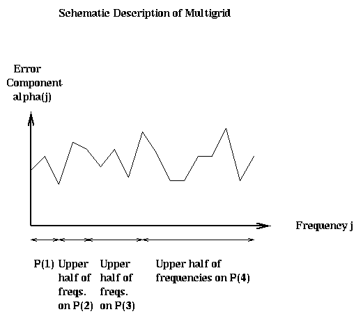
Using this terminology, we can describe Multigrid as follows. What Multigrid does on the finest grid P(m), is to damp down the upper half of the frequency components of the error in the solution. This is accomplished by the solution operator S(i), as we show below. On the next coarser grid, with half as many points, Multigrid damps the upper half of the remaining frequency components in the error. On the next coarser grid, the upper half of the remaining frequency components are damped, and so on, until we solve the exact (1 unknown) problem P(1). This is shown schematically below:
We begin by showing how the solution operation S(i) damps the upper half of the frequencies. S(i) can be described as "weighted Jacobi". Pure Jacobi would replace the j-th component of the approximate solution x(i) by the weighted average:
 improved x(i)(j)
         = .5*( x(i)(j-1) + x(i)(j+1) + 4^i * b(i)(j) )
         = x(i)(j) + .5*( x(i)(j-1) - 2*x(i)(j) +
                          x(i)(j+1) + 4^i * b(i)(j) )
Weighted Jacobi instead uses
 improved x(i)(j) = x(i)(j) +
     w*.5*( x(i)(j-1) - 2*x(i)(j) + x(i)(j+1) + 4^i * b(i)(j) )
where w is a weight. We will choose w to damp the highest frequencies;
w=2/3 turns out to be the right value, leading to the following definition
of S(i):
 improved x(i)(j) =
    (1/3)*( x(i)(j-1) + x(i)(j) + x(i)(j+1) + 4^i * b(i)(j) )
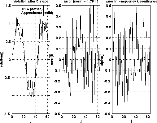
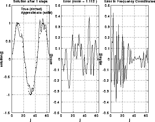
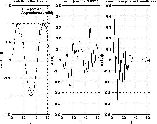
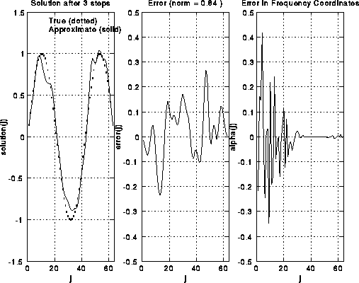
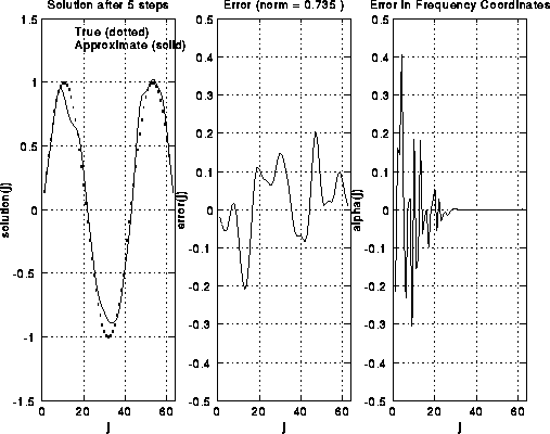
Here are some pictures to illustrate S(i). We take i=6, so there are 2^6-1=63
unknowns. There are 6 rows of pictures, the first row showing the
initial solution and error, and the following 5 rows showing the
solution and error after successive applications of S(i).
The true solution is a sine curve, shown as a dotted line
in the leftmost plot in each row. The approximate solution is a solid
line in the same plot. The middle plot shows the error alone, including
its norm in the title at the top.
The rightmost plot shows the frequency components of the error (V'*error).
One can see in the rightmost plots that as S(i) is applied,
the right (upper) half of the frequency components are damped out.
This can also be seen in the middle and left plots, because the approximate
solution grows smoother.
This is because high frequency error looks like "rough" error, and
low frequency error looks like "smooth" error. Initially, the norm
of the vector decreases rapidly, from 1.78 to 1.11, but then decays
more gradually, because there is little more error in the high frequencies
to damp. Thus, it only makes sense to do 1 or perhaps 2 iterations of S(i)
at a time.

For a more mathematical discussion of how weighted Jacobi damps the high frequencies, click here.
In 2D, S(i) requires each grid point be replaced by a similar weighted average of its 4 neighboring values in the grid.
Now we turn to the restriction operator R(i), which takes a problem P(i) with right-hand-side b(i), and an approximate solution x(i), and maps it to a simpler problem P(i-1) with right-hand-side b(i-1) and approximate solution x(i-1). The basic idea is as follows. Let r(i) be the residual of the approximate solution x(i):
r(i) = T(i)*x(i) - b(i)
If x(i) were the exact solution, r(i) would be zero. If we could solve the
equation
T(i) * d(i) = r(i)
exactly for the correction d(i), then x(i)-d(i) would be the solution
we seek, because
       T(i) * ( x(i)-d(i) ) = T(i)*x(i) - T(i)*d(i)
                            = (r(i) + b(i)) - (r(i))
                            = b(i)
Thus, to apply R(i) to ( b(i), x(i) ) and get P(i-1), we will
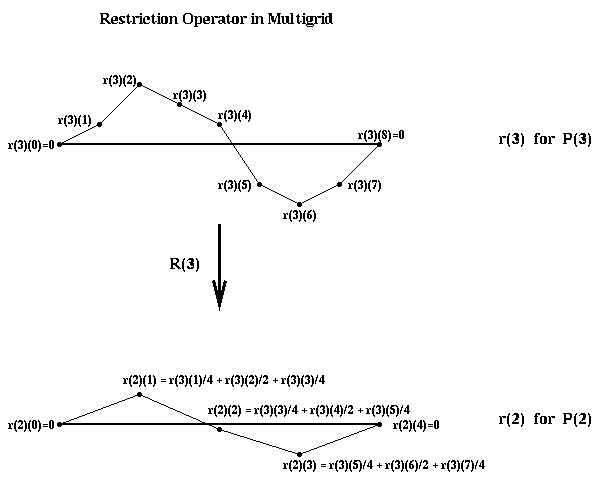
In 2D, R(i) requires averaging with up to 8 nearest neighbors (in the N, S, E, W, NW, SW, SE and NE compass directions).
Finally, the interpolation operator In(i-1) takes the solution of the residual equation T(i-1)*x(i-1) = r(i-1), and uses it to correct the fine grid approximation x(i) as described above. The solution x(i-1) is interpolated to the finer grid as shown below:
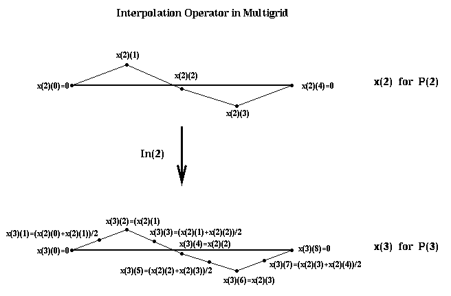
In 2D, interpolation requires averaging with up to 4 nearest neighbors (NW, SW, SE and NE).
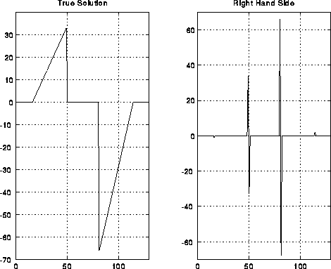
We close with some pictures of Multigrid working on a 1D problem, and then a 2D problem. The next graph is the right hand side and true solution for a 1D problem with 127=2^7-1 unknowns.
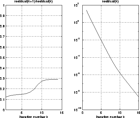
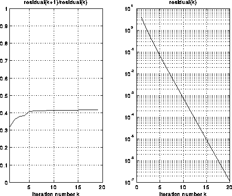
The next graphs summarize the convergence of Multigrid in two ways. The graph on the right shows the residual residual(k) = norm(T(i)x(i)-b(i)) after k iterations of Full Multigrid (FMG). The graph on the left shows the ratio of consecutive residuals, showing how the error (residual) is decreased by a factor bounded away from 1 at each step (for less smooth solutions, the residual will tend to decrease by a factor closer to .5 at each step.)
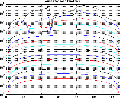
Finally, the following graph shows the error at each grid point in all iterations, with consecutive iterations plotted in different colors to distinguish them. We can see that eventually the errors change by a constant decrement on this semilog plot, which means they decrease by a constant factor. Also, we see that the error becomes much smoother as we continue to iterate.
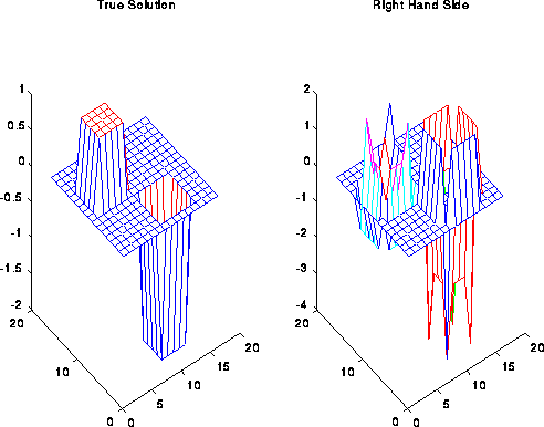
The following is a small 2D illustration. The first two graphs are the true solution and right hand side, and the next two plots shows the residuals as above.
We assume we have an n=(2^m+1)-by-n grid of data, and that p=s^2 is a perfect square. The data is laid out on an s-by-s grid of processors, with each processor owning an ((n-1)/s)-by-((n-1)/s) subgrid. This is illustrated in the following diagram by the pink dotted line, which encircles the grid points owned by the corresponding processor. The grid points in the top processor row have been labeled (and color coded) by the grid number i of the problem P(i) in which they participate. There is exactly one point labeled 2 per processor. The only grid point in P(1) with a nonboundary value is owned by the processor above the pink one. In general, if p>=16, there will be .5*log_2(p)-1 grids P(i) in which fewer than all processor own participating grid points.
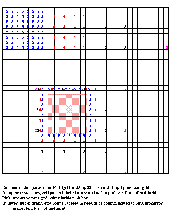
The processor indicated by the pink dotted line requires certain grid point data from its neighbors to execute the algorithm; this data has been indicated by the same color coded numbers as before. For example, to update its own (blue) grid points for P(5), the pink processor requires 8 blue grid point values from its N, S, E, and W neighbors, as well as single blue grid point values from its NW, SW, SE and NE neighbors. Similarly, updating the (red) grid points for P(4) requires 4 red grid point values from the N, W, E and W neighbors, and one each from the NW, SW, SE and NE neighbors. This pattern continues until each processor has only one grid point. After this, only some processors participate in the computation, requiring one value each from 8 other processors. This is enough to do a big-Oh analysis of the communication costs. For simplicity, let p=4^k=2^(2*k), so each processor owns a 2^(m-k)-by-2^(m-k) subgrid. Consider a V-cycle starting at level m. Then in levels m through k of the V-cycle, each processor will own at least one grid point. After that, in levels k-1 through 1, fewer than all processors will own an active grid point, and so some processors will remain idle. Let f be the time per flop, alpha the time for a message startup, and beta the time per word to send a message.
At level m >= i >= k, the time in the V-cycle will be
 Time at level i = O( 4^(i-k) ) * f
                       ... number of flops, proportional to the
                       ... number of grid points per processor

                 + O( 1 ) * alpha
                       ... send a constant number of messages
                       ... to neighbors

                 + O( 2^(i-k) ) * beta
                       ... number of words sent
Summing all these terms from i=k to m yields
  Time at levels k to m = O( 4^(m-k) )*f +
                          O( m-k )*alpha +
                          O( 2^(m-k) )*beta

                        = O( n^2/p )*f +
                          O( log(n/p) )*alpha +
                          O( n/sqrt(p) )*beta
Note that there is a "surface-to-volume effect" when i>>k, with each processor
communicating just its boundary data and computing with the many more
grid points that it owns.
We have seen this attractive phenomenon before in particle
simulations, where it also meant that computation time was likely to dominate
communication time.
On levels k >= i >= 1, this effect disappears, because each processor needs to communicate about as many words as it does floating point operations:
 Time at level i = O( 1 ) * f
                      ... number of flops, proportional to the
                      ... number of grid points per processor

                 + O( 1 ) * alpha
                      ... send a constant number of messages
                      ... to neighbors

                 + O( 1 ) * beta
                      ... number of words sent
Summing all these terms yields
  Time at levels 1 to k-1 = O( k-1 )*f +
                            O( k-1 )*alpha +
                            O( k-1 )*beta

                          = O( log(p) )*f +
                            O( log(p) )*alpha +
                            O( log(p) )*beta
The total time for a V-cycle starting at the finest level is therefore
  Time = O( n^2/p + log(p) )*f +
         O( log(n) )*alpha +
         O( n/sqrt(p) + log(p) )*beta
Similarly, the total time for a V-cycle starting at level j, k <= j <= m, is
  Time(j) = O( 4^j/p + log(p) )*f +
            O( j )*alpha +
            O( 2^j/sqrt(p) + log(p) )*beta
The total time for a V-cycle starting at level j < k is
  Time(j) = O( j )*f +
            O( j )*alpha +
            O( j )*beta
Therefore, the total time for Full Multigrid, assuming n^2 >= p,
so that each processor has at least 1 grid point, is
  Time = sum_{j=1}^m Time(j)

       = O( n^2/p + log(p)*log(n) )*f +
         O( (log(n))^2 )*alpha +
         O( n/sqrt(p) + log(p)*log(n) )*beta

       = O( N/p + log(p)*log(N) )*f +
         O( (log(N))^2 )*alpha +
         O( sqrt(N/p) + log(p)*log(N) )*beta
where N=n^2 is the number of unknowns.
Thus we see that the speedup of the serial floating point work O(N), is
nearly perfect, O( N/p + log(p)*log(N) ), when N>>p, but reduces to
log(N)^2 when p=N (the PRAM model).
In practice, the time spent on the coarsest grids, when each processor has one or zero active grid points, while negligible on a serial machine, is significant on a parallel machine, enough so to make the efficiency noticeably lower. For example, in the paper "Analysis of the Multigrid FMV Cycle on large scale parallel machines", R. Tuminaro and D. Womble, SIAM J. Sci. Comp. v. 14, n. 5, 1993, the authors consider several variations of multigrid on a 1024 processor nCUBE2. This machine has a relatively low latency and high bandwidth compared to its floating point speed. On a 64-by-64 grid of unknowns, where there are only 4 unknowns per processor on the finest grid, (this is quite small for such a large machine!), the efficiency of a V-cycle alone was .02, and for Full Multigrid it was .008. In this case, most of the time some processors are idle. For a 1024-by-1024 grid, with 1024 unknowns per processor, the efficiencies were .7 and .42, respectively, which are quite reasonable, though Full Multigrid is noticeably less efficient. Still, it is 2.6 times faster than V-cycles alone for solving the problem. The authors explored variations on Full Multigrid, where they did varying numbers of calls to MGV (a V-cycle) within the loop of FMG, using estimates of convergence rate and parallel efficiencies to pick the optimal number of MGV calls; they were able to increase the efficiencies to .01 and .47, respectively. For the 1024-by-1024 grid, either efficiency (.42 or .47) is quite reasonable.
            # flops        # messages   # words sent

SOR         N^(3/2)/p      N^(1/2)      N/p

FFT         N*log(N)/p     p^(1/2)      N/p

Multigrid   N/p +          (log(N))^2   (N/p)^(1/2) +
            log(p)*log(N)               log(p)*log(N)
SOR is slower than the other two methods on all counts. It is hard to say whether the number of flops for FFT or Multigrid is smaller, because the number of Full Multigrid iterations depends on how much accuracy is desired, whereas the FFT only delivers full accuracy. Multigrid sends clearly fewer words than the FFT or SOR.
However, it is not clear whether the FFT or Multigrid sends fewer messages. The number of messages is a much more slowly growing function of N than either the number of flops or the number of words sent, and for large enough N it will be overwhelmed by these terms. But if the cost per message, alpha, is large enough, and p is small, it is not clear whether the FFT or Multigrid is faster; this big-Oh analysis is not sufficient to distinguish them, and the answer will depend on details of the machine and implementation.