CS267: Lecture 14, Feb 29, 1996

Design and Implementation of LAPACK and ScaLAPACK

Table of Contents

Overview of LAPACK and ScaLAPACK

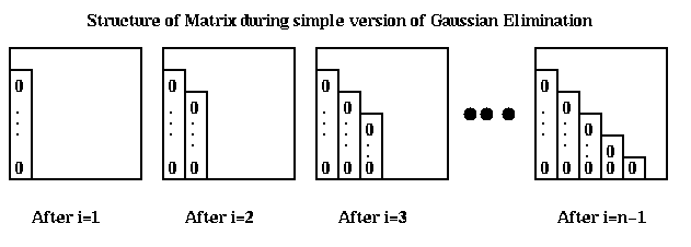
We will outline the contents of these libraries, and discuss the design of the basic linear equation solver in some detail. The major issues will include

We will use Matlab notation to express our algorithms below. Recall that

The 6 most basic problem of linear algebra are summarized below. For details, see any good text book in numerical linear algebra, such as "Matrix Computations" by Golub and Van Loan, or "Numerical Linear Algebra" by J. Demmel. Lectures 11, 12 and 13 describe how some of these problems arise in doing simulations of physical systems.

         A*x_i = lambda_i * x_i,

       A = U*S*V'.
  

The most important determiner of which algorithm to use for these problems is whether the matrix A is dense or sparse. A dense matrix has all (or mostly) nonzero entries, without any special properties that would let one represent using many fewer than n^2 independent numbers. Sparse matrices either have lots of zero entries, or are otherwise much more compactly representable than n^2 numbers. The algorithms for sparse matrices, which are very common in science and engineering, are often rather different than algorithms for dense matrices, and we will discuss them in detail in other lectures.

For a small example of a sparse matrix, click here. The first picture is a mesh around a wing. The physical problem is to compute the airflow around the wing at the mesh points. This leads to solving a sparse n-by-n system of spd linear equations Ax=b, where n=4253 and A has the "sparsity structure" in the top left plot of the second picture (black dots represent nonzero entries, the rest are zero). Only .16% of the 4253^2 entries of A are nonzero. The top right plot of the second picture is a different view of the matrix, with the rows and columns permuted. If we did Gaussian elimination on the spd matrix A without taking sparsity into account, it would take (1/3)*n^3 = 2.6e10 floating point operations. If we do Gaussian elimination on the matrix in the top left, and take sparsity into account by not doing unnecessary operations on zero entries, it does over 2200 times fewer operations, resulting in the Cholesky factor at the bottom left. If we do Gaussian elimination on the matrix at the top right, we get the Cholesky factor at the bottom right for 4 times fewer operations still. This matrix is available in matlab by typing demo, and clicking on

The next important distinction among linear algebra problems is between the first two problems (solving Ax=b and least squares problems), and the last problem (computing eigenvalues and the SVD). The first two problems have exact, finite solution procedures, and the latter can only be solved approximately. The first two problems have exact finite solutions in the sense that algorithms doing O(n^3) operations exist for each, which would yield the exact solution in the absence of round-off errors. (Analyzing roundoff is a topic for a numerical analysis class, and we will only mention it here when it requires us to modify the algorithm to make it reliable.) In contrast, to compute eigenvalues requires iterative solutions, because they implicitly require finding the roots of the characteristic polynomial of the matrix A: p(x)=determinant(A-x*I) (for the SVD substitute A'*A for A). As shown by Galois, no finite algorithm can exist to find the roots of a general polynomial of degree 5 or greater. A large variety of iterative solutions exist. In practice, the best iterations converge so reliably and so rapidly (quadratically, where the error is squared at every step, or even cubically) that they are often considered to be finite solutions.

Eigenvalue and singular value problems are all solved in 2 phases: a (finite) algorithm to reduce the original dense matrix to a more compactly representable form with the same eigenvalues (or singular values), and an iterative phase on the compact form. We will again distinguish the first two problems from the initial phases of the latter problems: For the first two problems, it is known how to do almost all the work by using matrix-matrix multiplication (BLAS3), which according to Lecture 2 is the fastest available linear algebra building block. In contrast, the first phases of the latter problems are more difficult to convert to BLAS3. The algorithm in LAPACK does 50% of its work in the BLAS3 and 50% in the slower matrix-vector multiplication (BLAS2). More recently, work on "multi-step band-reduction" by C. Bischof, X. Sun, and others has shown that if no eigenvectors are desired, one can use nearly 100% BLAS3. If eigenvectors are desired, one either has to use BLAS2 or increase the operation count significantly (by 2n^3).

In other words, we can in principle take nearly full advantage of the memory hierarchy for the first two problems, but not the latter ones, at least if eigenvectors are desired and we do not want to increase the operation count significantly.

Now consider just eigenvalue and singular value problems. The iterative phase of finding the eigenvalues of a general matrix is much more expensive than the initial reduction phase. In contrast, the best recent iterations for the symmetric eigenvalue problem and SVD are in principle much cheaper than the corresponding reduction phases (this was not true until recently).

Good parallel software for the first two problems exists in LAPACK and ScaLAPACK. Software for eigenvalue and singular value problems exists in LAPACK, with recent better algorithms on the way. ScaLAPACK currently only solves the symmetric eigenproblem, and the Feb 1995 release makes certain unfortunate compromises between parallel efficiency and accuracy, which future algorithms should make unnecessary. Class projects to improve and expand ScaLAPACK are available.

It is interesting to ask whether the best parallel algorithm is always a parallel version of the best serial algorithm. This is usually the case, and in fact the search for better parallel algorithms has sometimes led to better serial algorithms as well. However, there are some interesting exceptions. For example, certain "banded" linear systems can be solved more quickly using parallel-prefix than Gaussian elimination, but the results are numerically unstable in the presense of roundoff, and so potentially much less accurate. Currently, LAPACK and ScaLAPACK use different algorithms for finding eigenvalues, but we expect them to use the same algorithm eventually, once we better understand the problem.

Quick review of Gaussian Elimination

Gaussian elimination to solve Ax=b starts with a dense matrix, and adds multiples of each row to subsequent rows in order to create zeros below the diagonal, ending up with an upper triangular matrix we will call U. Then, one solves a linear system with U, which can be done by substitution starting with the last variable. The simplest way one could write this algorithm is as follows, where we ignore transformations of b for the time being:

 ... for each column i,
 ... zero it out below the diagonal by
 ... adding multiples of row i to later rows
 for i = 1 to n-1
     ... each row j below row i
     for j = i+1 to n
         ... add a multiple of row i to row j
         for k = i to n
             A(j,k) = A(j,k) -
                     (A(j,i)/A(i,i)) * A(i,k)

Let us improve this rudimentary implementation step by step. First, we remove the constant (A(j,i)/A(i,i)) from the innermost loop:

  for i = 1 to n-1
    for j = i+1 to n
        m = A(j,i)/A(i,i)
        for k = i to n
           A(j,k) = A(j,k) - m * A(i,k)

Next, we avoid computing results we know, i.e. the zeros below the diagonal:

  for i = 1 to n-1
    for j = i+1 to n
        m = A(j,i)/A(i,i)
        for k = i+1 to n
            A(j,k) = A(j,k) - m * A(i,k)

It will be convenient to store the multipliers m in the implicitly created zeros below the diagonal, so we can use them later to transform the right hand side b:

  for i = 1 to n-1
    for j = i+1 to n
        A(j,i) = A(j,i)/A(i,i)
    for j = i+1 to n
        for k = i+1 to n
            A(j,k) = A(j,k) - A(j,i) * A(i,k)

Now we use Matlab notation to express the algorithm even more compactly. Note that the last two loops are really multiplying the column vector A(i+1:n, i) times the row vector A(i, i+1:n), and add the resulting (n-i)-by-(n-i) matrix to A(i+1:n, i+1:n):

  for i = 1 to n-1
    A(i+1:n, i) = A(i+1:n, i) / A(i,i)
    A(i+1:n, i+1:n) = A(i+1:n, i+1:n) -
                      A(i+1:n, i)*A(i, i+1:n)

Thus, the inner loop consists of one BLAS1 operation (scaling A(i+1:n,i) by a constant), and one BLAS2 operation (adding a rank-one matrix -A(i+1:n,i)*A(i,i+1:n), to A(i+1:n, i+1:n)). Here is a picture of what happens at step i.

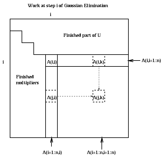
Call the strictly lower triangular matrix of multipliers which is stored below the diagonal of A after the algorithm ends M, and let L=I+M. Recall that U is the upper triangular matrix stored in the upper triangular of A. We state the following easy lemma without proof.

Lemma. (LU Factorization). If the above algorithm terminates (i.e. it did not try to divide by zero) then A = L*U.

Now we can state our complete algorithm for solving A*x=b:

   1) Factorize A = L*U.
   2) Solve L*y = b for y 
         by forward substitution.
   3) Solve U*x = y for x 
         by backward substitution.

Then x is the solution we seek because A*x = L*(U*x) = L*y = b.

Let us compute the serial and PRAM complexity of this algorithm. From the matlab code, it is easy to see that the number of floating point operations performed (serial complexity) is

 sum_{i=1}^{n-1}
     [ (n-i)
       ... cost of A(i+1:n,i+1:n)/A(i,i),
       + 2*(n-i)^2 ]
       ... cost of A(i+1:n,i+1:n) -
       ...         A(i+1:n,i)*A(i,i+1:n).
   = (2/3)*n^3 + O(n^2)

Solving L*y=b and U*x=b each only cost n^2, so the total cost is still (2/3)*n^3 + O(n^2).

Assuming we have one processor per matrix entry, and that communication is free (the PRAM model), the cost is

 sum_{i=1}^{n-1}
     [ 1
       ... cost of A(i+1:n,i+1:n)/A(i,i)
       + 2 ]
       ... cost of A(i+1:n,i+1:n) -
       ... A(i+1:n,i)*A(i,i+1:n)
   = 3*(n-1)

since all the divisions in the inner loop can be done at once, all the multiplications can be done at once, and all the subtractions can be done at once. Thus, a lot of parallelism is available in this algorithm for us to exploit. One can also confirm that solving L*y=b and U*x = y in straightforward ways:

 ... in practice, y is overwritten on b
 y(1:n) = b(1:n)
 for i = 1 to n-1
    y(i+1:n) = y(i+1:n) - y(i)*L(i+1:n,i)

 ... in practice, x is overwritten on y, 
 ... i.e. on b
 x(1:n) = y(1:n)
 for i = n downto 1
    x(i) = x(i)/U(i,i)
    x(1:i-1) = x(1:i-1) - x(i)*U(1:i-1,i)

costs (1+2*(n-1)) + (1+n+2*(n-1)) = 5n-2, for a grand total of 8*n-5. Interestingly, in the PRAM model, solving triangular systems with the most straigthtforward algorithms is about as expensive as LU factorization, whereas triangular system solving was much cheaper on a serial machine.

Here are some obvious problems with this algorithm, which we need to address:

Pivoting to avoid tiny A(i,i)

     A= [ 0 1 ]
        [ 1 0 ]

     A= [ 1e-4  1 ]  and  b= [ 1 ]  .
        [  1    1 ]          [ 2 ]

     x = [ 1 ]  .
         [ 1 ]

   L = [    1        0 ]  =  [  1   0 ]
       [ fl(1/1e-4)  1 ]     [ 1e4  1 ]
       ... no error yet
 and
   U = [ 1e-4      1      ] = [ 1e-4   1  ]
       [  0   fl(1-1e4*1) ]   [  0   -1e4 ]
       ... error in the 4th place

     L * U = [  1e-4   1  ]
             [   1     0  ]

   y = [      1      ] = [   1  ]
       [ fl(1-1e4*1) ]   [ -1e4 ]
       ... error in the 4th place
 and
   x = [ x1 ] = [ fl((1-x2*1)/1e-4) ] 
       [ x2 ]   [  fl(-1e4/(-1e4))  ]   
     = [ 0 ]
       [ 1 ]
       ... no error in either component

  Gaussian elimination with Partial Pivoting,
    BLAS2 implementation

  for i = 1 to n-1
    find and record k where 
       |A(k,i)| = max_{i<=j<=n} |A(j,i)|
    if |A(k,i)|=0, exit with a warning
       that A is singular, or nearly so
    if i != k, swap rows i and k of A
    A(i+1:n, i) = A(i+1:n, i) / A(i,i)
    ...  each quotient lies in [-1,1]
    A(i+1:n, i+1:n) = A(i+1:n, i+1:n) -
                  A(i+1:n, i)*A(i, i+1:n)

The LAPACK source for this routine, sgetf2, may be viewed by clicking here.

We may describe this algorithm as computing the factorization P*A=L*U, where L and U are lower and upper triangular as before, and P is a permutation matrix, i.e. the identity matrix with permuted columns. P*A is the matrix A with its rows permuted. As a consequence of pivoting, each entry of L has absolute value at most 1. Using this new factorization of A, solving A*x=b only requires the additional step of permuting b according to P.

Note that we have several choices as to when to swap rows i and k. Indeed, we could use indirect addressing and not swap them at all, but then we couldn't use the BLAS, so this would be slow. Different implementations make different choices about when to swap.

How to Use BLAS3 in Gaussian Elimination with Partial Pivoting

For LU decomposition, this means that we will process the matrix in blocks of b columns at a time, rather than one column at a time. b is called the block size. We will do a complete LU decomposition just of the b columns in the current block, essentially using the above BLAS2 code. Then we will update the remainder of the matrix doing b rank-one updates all at once, which turns out to be a single matrix-matrix multiplication, where the common matrix dimension is b. b will be chosen in a machine dependent way to maximize performance. A good value of b will have the following properties:

 Gaussian elimination with Partial Pivoting,
    BLAS3 implementation

 ... process matrix b columns at a time
 for ib = 1 to n-1 step b
    ... point to end of block of b columns
    end = min(ib+b-1,n)

    ... LU factorize A(ib:n,ib:end) with BLAS2
    for i = ib to end
       find and record k where
          |A(k,i)| = max_{i<=j<=n} |A(j,i)|
       if |A(k,i)|=0, exit with a warning
          that A is singular, or nearly so
       if i != k, swap rows i and k of A
       A(i+1:n, i) = A(i+1:n, i) / A(i,i)
       ... only update columns i+1 to end
       A(i+1:n, i+1:end) = A(i+1:n, i+1:end)
                 - A(i+1:n, i)*A(i, i+1:end)
    endfor
        
    ... Let LL be the b-by-b lower triangular
    ... matrix whose subdiagonal entries are
    ... stored in A(ib:end,ib:end), and with
    ... 1s on the diagonal. Do delayed update 
    ... of A(ib:end, end+1:n) by solving 
    ... n-end triangular systems
    ... (A(ib:end, end+1:n) is pink below)
    A(ib:end, end+1:n) = 
                  LL \ A(ib:end, end+1:n)

    ... do delayed update of rest of matrix
    ... using matrix-matrix multiplication
    ... (A(end+1:n, end+1:n) is green below)
    ... (A(end+1:n, ib:end) is blue below)
    A(end+1:n, end+1:n) = A(end+1:n, end+1:n)
        - A(end+1:n,ib:end)*A(ib(end,end+1:n)

 endfor

The LU factorization of A(ib:n,ib:end) uses the same algorithm as before. Solving a system of n-end equations with triangular coefficient matrix LL is a single call to a BLAS3 subroutine (strsm) designed for that purpose. No work or data motion is required to refer to LL; it is done with a pointer. When n>>b, almost all the work is done in the final line, which multiplies an (n-end)-by-b matrix times a b-by-(n-end) matrix in a single BLAS3 call (to sgemm). Here is a picture, where the final line subtracts the product of the blue and pink submatrices from the green submatrix.

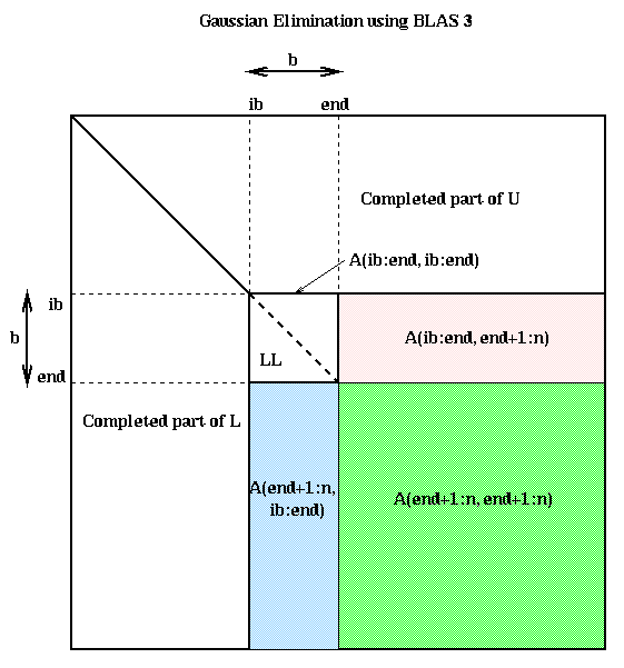
Here is another way to derive this algorithm. Suppose that we are at the top of the ib loop, midway through the algorithm. Then implicitly we have computed the following factorization, where all the submatrices are the same size as in the above figure (for simplicity we ignore pivoting):

        ib-1   b  n-b-ib
 ib-1  [ A11  A12  A13  ]
  b    [ A21  A22  A23  ]
n-b-ib [ A31  A32  A33  ]

       [ L11  0  0 ]   [ U11 U12  U13  ]
     = [ L21  I  0 ] * [  0  A'22 A'23 ]
       [ L31  0  I ]   [  0  A'32 A'33 ]

    [ A11  A12  A13  ]
    [ A21  A22  A23  ]
    [ A31  A32  A33  ]

    [ L11  0  0 ]   [ U11   U12   U13  ]
  = [ L21  I  0 ] * [  0  L22*U22 A'23 ]
    [ L31  0  I ]   [  0  L32*U22 A'33 ]

    [ A11  A12  A13  ]
    [ A21  A22  A23  ]
    [ A31  A32  A33  ]

    [ L11  0  0 ]   [ U11   U12     U13   ]
  = [ L21  I  0 ] * [  0  L22*U22 L22*U23 ]
    [ L31  0  I ]   [  0  L32*U22   A'33  ]

    [ A11  A12  A13  ]
    [ A21  A22  A23  ]
    [ A31  A32  A33  ]

    [ L11  0  0 ]   
  = [ L21 L22 0 ] 
    [ L31 L32 I ]   

      [ U11  U12       U13        ]
    * [  0   U22       U23        ]
      [  0    0   A'33 - L32*U23  ]

    [ L11  0  0 ]   [ U11  U12  U13   ]
  = [ L21 L22 0 ] * [  0   U22  U23   ]
    [ L31 L32 I ]   [  0    0   A''33 ]

The LAPACK source for this routine, sgetrf, may be viewed by clicking here.

Performance of LAPACK LU Decomposition

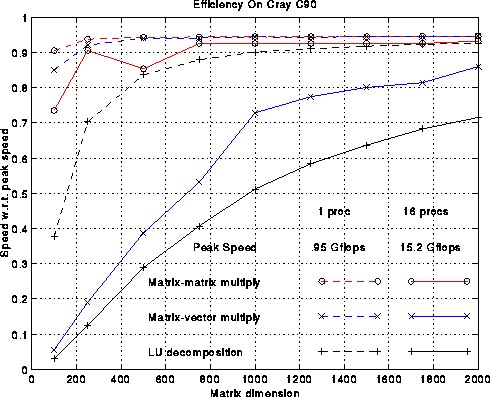
Now we fix the dimension at N=1000 and compare the efficiencies on a variety of architectures, from large vector processors like the Cray C90 and Convex C4640, to shared-memory multiple processor versions of both machines, to workstations like the DEC Alpha, IBM RS6000/590, and SGI Power Challenge. The vital statistics of these machines are given in the following table. All results are for 64-bit precision.

Machine          #Procs  Clock    Peak  Block
                         Speed  Mflops Size b
                         (MHz)
---------------------------------------------
Convex C4640          1    135     810     64
Convex C4640          4    135    3240     64
Cray C90              1    240     952    128
Cray C90             16    240   15238    128
DEC Alpha 3000-500X   1    200     200     32
IBM RS 6000/590       1     66     264     64
SGI Power Challenge   1     75     300     64

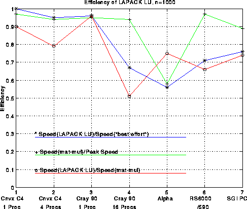
Now consider the red line, which is the speed of LU decomposition divided by the speed of matrix-multiply. The block size b is given in the above table; it was chosen by brute force search to optimize the performance. This curve measures how well we achieved our goal of making LU decomposition as fast as the matrix-multiply in its inner loop. The best efficiency, 95%, is attained on a single processor Cray C90, and the worst efficiency, 50%, is attained on a 16 processor Cray C90. This drop in performance is due to the fact that multiplying (n-i)-by-128 times 128-by-(n-i) matrices does not yield enough work to keep all 16 processors busy, although it is enough for 1 processor. The workstations (Alpha, RS6000, SGI) are all close to 70% efficient, which is reasonably satisfactory.

Finally, the blue line measures the efficiency of our LU decomposition with respect to "best effort", which means a version of LU decomposition crafted by each vendor especially for its machine. These vendor-supplied codes use very similar techniques to the ones described above, but try to improve performance by using a variable block size, assembly language, or an algorithm corresponding to a different permutation of the 3 nested loops in the original algorithm (all 3!=6 permutations lead to viable algorithms). The blue curve measures the extent to which we have sacrificed performance to gain portability: We have not lost much on the large vector machines, but 25%-30% on the workstations. The vendors typically invest a large amount of effort in optimizing 1000-by-1000 LU because it is one of the most popular benchmarks used to compare high performance machines: the LINPACK Benchmark. It would be nice if vendors had the resources to highly optimize all the library routines one might want to use, but few do, so portable high-performance libraries remain of great interest.

The LINPACK Benchmark is named after the predecessor of LAPACK. It originally consisted just of timings for 100-by-100 matrices, solved using a fixed Fortran program (sgefa) from the LINPACK linear algebra library. The data is an interesting historical record, with literally every machine for the last 2 decades listed in decreasing order of speed, from the largest supercomputers to a hand-held calculator. As machines grew faster and vendors continued to optimize their LINPACK benchmark performance (sometimes by using special compiler flags that worked only for the LINPACK benchmark!), the timings for 100-by-100 matrices grew less and less indicative of typical machine performance. Then 1000-by-1000 matrices were introduced. In contrast to the 100-by-100 case, which required vendors to use identical Fortran code, vendors were permitted to modify Gaussian elimination anyway they wanted for the 1000-by-1000 case, provided they got an accurate enough answer. Finally, a third benchmark was added for large parallel machines, which measured their speed on the largest linear system that would fit in memory, as well as the size of the system required to get half the Mflop rate of the largest matrix.

Here is a plot analogous to the last one but for 100-by-100 matrices. Generally speaking, efficiencies are lower for n=100 than n=1000, dramatically so for large machines like the Cray, less so for workstations. Rather than comparing LAPACK performance to the ``best effort'', it is compared to the LINPACK benchmark discussed above, i.e. performance using the LINPACK benchmark code sgefa. This ratio is as high as 2.46 for, but is as low as .73, a testimony to the efforts of the manufacturers to tune their compilers to work well on sgefa.

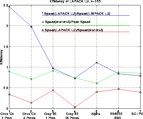
For an analysis and summary of the performance of other LAPACK routines besides LU, click here.

How to Layout Matrices on Distributed Memory Machines

The two main issues in choosing a data layout for Gaussian elimination are

For convenience we will number the processors from 0 to p-1, and matrix columns (or rows) from 0 to n-1. The following figure shows a sequence of data layouts we will consider. In all cases, each submatrix is labeled with the number of the processor (from 0 to 3) that contains it. Processor 0 owns the shaded submatrices.

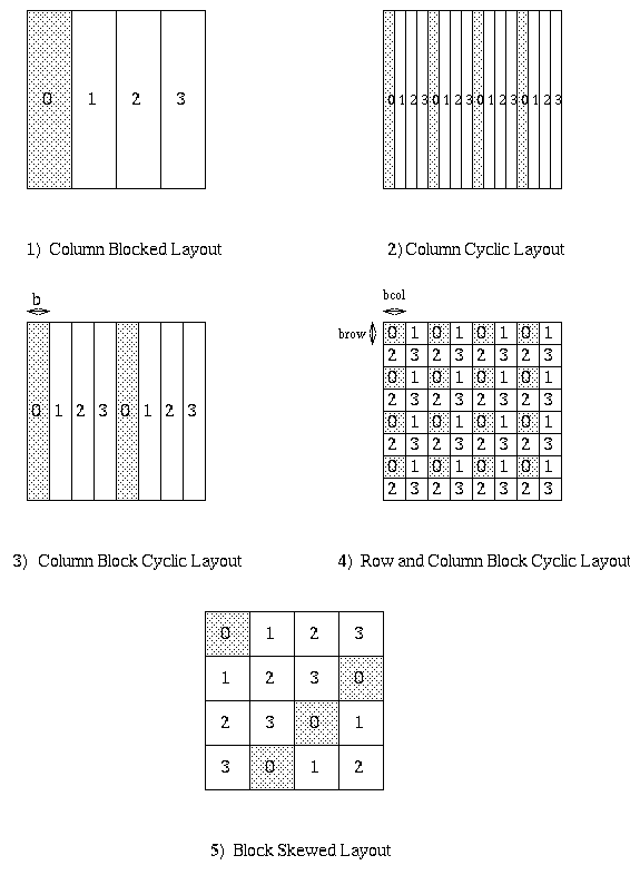
Consider the first layout, the Column Blocked Layout. In this layout, column i is stored on processor floor(i/c) where c=ceiling(n/p) is the maximum number of columns stored per processor. In the figure n=16 and p=4. This layout does not permit good load balancing, because as soon as the first c columns are complete, processor 0 is idle for the rest of the computation. The transpose of the this layout, the Row Blocked Layout, has a similar problem.

The second layout, the Column Cyclic Layout, tried to address this problem by assigning column i to processor i mod p. In the figure, n=16 and p=4. With this layout, each processor owns approximately 1/p-th of the square southeast corner of the matrix, so the load balance is good. However, the fact that single columns are stored rather than blocks means we cannot use the BLAS2 to factorize A(ib:n,ib:end), and may not be able to use the BLAS3 to update A(end+1:n,end+1:n). The transpose of this layout, the Row Cyclic Layout, has a similar problem.

The third layout, the Column Block Cyclic Layout, is a compromise between the last two. We choose a block size b, divide the columns into groups of size b, and distribute these groups in a cyclic manner. This means column i is stored in processor (floor(i/b)) mod p. In fact, this layout includes the first two as the special cases b=c=ceiling(n/p) and b=1, respectively. In the figure n=16, p=4 and b=2. For b larger than 1, this has a slightly worse balance than the Column Cyclic Layout, but can use the BLAS2 and BLAS3. For b less than c, it has a better load balance than the Columns Blocked Layout, but can only call the BLAS on smaller subproblems, and so perhaps take less advantage of the local memory hierarchy (recall our plot of performance of the BLAS3, where performance improved for larger matrix sizes). However, this layout has the disadvantage that the factorization of A(ib:n,ib:end) will take place on perhaps just on processor (in the natural situation where column blocks in the layout correspond to column blocks in Gaussian elimination). This would be a serial bottleneck.

This serial bottleneck is eased by the fourth layout in the figure, the Row and Column (or 2D) Block Cyclic Layout. Here we think of our p processors arranged in an prow-by-pcol rectangular array of processors, indexed in a 2D fashion by (pi,pj), 0 <= pi < prow and 0 <= pj < pcol. All the processors (i,j) with a fixed j are referred to as processor column j. All the processors (i,j) with a fixed i are referred to as processor row i. Matrix entry (i,j) is mapped to processor (pi,pj) by mapping i to pi and j to pj independently using the formula for a block cyclic layout:

    pi = floor(i/brow) mod prow, where 
  brow = block size in the row direction

    pj = floor(j/bcol) mod pcol, where 
  bcol = block size in the column direction

Since Gaussian elimination is not entirely "symmetric" (there is more communication required during the BLAS2 factorization of A(ib:n,ib:end) than during the BLAS3 update of A(ib:end,end+1:n)), it is not clear that choosing an entirely symmetric layout (prow=pcol) is most efficient. Indeed, later we will see that choosing prow There is one more layout shown, the Block Skewed Layout, which is not a special case of 2D Block Cyclic Layout. This layout has feature that each row and each column is shared among all p processors, so p-fold parallelism is available for any row operation or any column operation. In contrast, the 2D block cyclic layout can have at most sqrt(p)-fold parallelism in all the rows and all the columns. The Block Skewed Layout is not useful for Gaussian elimination, but can be useful in a variety of other matrix operations, so we mention it here.

Distributed Gaussian elimination with a 2D Block Cyclic Layout

The following figure shows how the BLAS3 algorithm is performed on a 2D block cyclic layout. The block size b in the algorithm and the block sizes brow and bcol in the layout satisfy b=brow=bcol. Shaded regions indicate busy processors or communication performed.

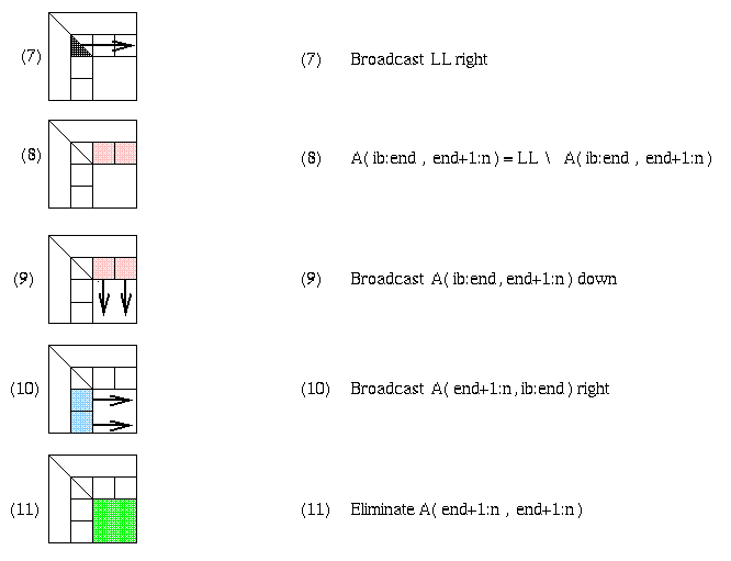
For example, step (1) requires a reduction operation among the prow processors owning the current column, in order to find the largest absolute entry (pivot) and broadcast its index. Step (2) requires communication among processors in that column to exchange rows, and broadcast the pivot row to all processors in the column. Steps (3) and (4) are local computation, BLAS1 and BLAS2, respectively. Steps (5) and (6) involve communication, broadcasting pivot information and swapping rows among all the other p-prow processors. Step (7) is more communication, sending LL to all pcol processors in its row. Step (8) is local computation. Steps (9) and (10) are communication, sending matrix blocks right and down respectively, in preparation for the local matrix multiplies that update the trailing southeast square matrix in step (11).

It is unnecessary to have a barrier between each step of the algorithm. In other words, there can be parallelism with some steps of the algorithm forming a pipeline. For example, consider steps 9, 10 and 11, where most of the communication and floating point work occurs. As soon as a processor received its desired (blue) subblock of A(end+1:n,ib:end) from the left, and (pink) subblock of A(ib:end:end+1:n) from above, it may begin its local matrix multiply to update its part of the (green) submatrix A(end+1:n,end+1:n). As soon as the leftmost b columns of A(end+1:n,end+1:n) are updated, their LU factorization may begin while the remaining columns of the green submatrix are being updated by other processors.

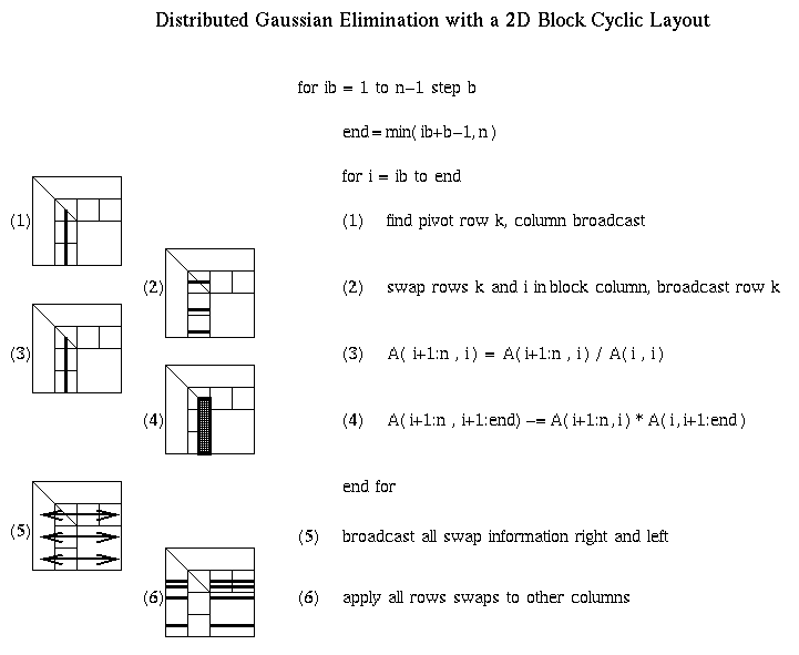
The ScaLAPACK software which implements this is located here. To view the top level routine that performs Gaussian elimination, pdgetrf.f, click here.

Modeling the Performance of Distributed Gaussian Elimination

   Time =   msgs * alpha 
          + words * beta + flops   time units

The implementation we discuss will overlap steps 10 and 11 of the algorithm as described above. More precisely,

    Time for step 9 = 
         ( log_2 prow ) * 
         ( alpha + (b*(n-end)/pcol)*beta )
         time units

    ( pcol ) * 
    ( alpha + (b*(n-end)/prow)*beta ) 
    time units.

    Time for step 10 = 
        2 * ( alpha + (b*(n-end)/prow)*beta ) 
        time units.

    Time for step 11 = 2*b*(n-end)^2/p 
                       time units.

 Time for all steps 9, 10 11 =   
       ( ( n * (log_2 prow) + 2 ) / b )
         * alpha
     + ( n^2 * 
         ( (log_2 prow)/(2*pcol) + 1/prow ) 
       ) * beta
     + ( (2/3)*n^3/p )

 Time for distributed Gaussian elimination =
       ( n * (6+ log_2 prow) ) * alpha
     + ( n^2 *
         ( 2*(prow-1)/p + 
           (pcol-1)/p + 
           (log_2 prow)/(2*pcol) 
         )
       ) * beta
     + ( (2/3)*n^3/p )

  Efficiency = 1 / (  1 
     + (1.5*p*(6 + log_2 prow)/n^2) 
       * alpha
     + ( 1.5*
       ( 2*prow + pcol 
         + (prow * log_2 prow)/2 -3 ) 
       /n )
       * beta )

Now we consider the choice of prow and pcol. The expression

   2*prow + pcol + (prow * log_2 prow)/2  
      = 2*prow +p/prow + (prow * log_2 prow)/2

Overall, assuming prow ~ pcol ~ sqrt(p), and ignoring the log terms, the efficiency is

  Efficiency = 1 / ( 1 + O( p/n^2 * alpha ) +
                  O( sqrt(p)/n * beta ) )
             = E( n^2/p )

We will use the Intel Gamma, which has the following machine parameters:

        p    prow     pcol
      ---    ----     ----
        1      1        1
       16      4        4
       32      4        8
       64      8        8
      128      8       16

Software Structure of ScaLAPACK

A great deal of software infrastructure is needed to implement the ScaLAPACK algorithms described above. As we have said in previous lectures, the design goal is to build software layers that hide the details of lower levels, and so make it simple to write (and debug and maintain) software at higher levels. In this section we will describe the layers inside ScaLAPACK. They are depicted in the figure below:

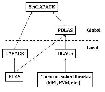
Below the dotted line is local software, and above the dotted line is global software. Local software either only runs on one processor, and is not parallel, or refers to other processors explicitly to do communication. Global software refers to data structures, and operations on them, that are spread out over the whole parallel machine (or selected subsets).

We have already discussed the BLAS, or Basic Linear Algebra Subroutines, at length in Lecture 2, and will not dwell on them here. The use of the BLAS, especially BLAS3, in LAPACK is discussed above. Neither the BLAS nor LAPACK are explicitly parallel.

(We note that on shared memory parallel machines, it is possible to hide all the parallelism within the BLAS, by doing matrix-matrix multiplication in parallel for example, and so to run LAPACK in parallel without changing any software. The extra complexities of ScaLAPACK are due to the lack of a shared address space. Also, there are some LAPACK routines for eigenvalue problems, whose ScaLAPACK counterparts use different algorithms. We discuss these in other lectures.)

The BLACS are the Basic Linear Algebra Communication Subroutines. These routines are message passing libraries which let the user send, receive, broadcast, reduce and do other basic operations on the matrix data types used in ScaLAPACK algorithms, namely rectangular or trapezoidal matrices, and submatrices of other matrices. The BLACS hide (almost all!) the differences between the underlying message passing libraries (PVM, MPI, MPL for the IBM SP-1 and SP-2, CMMD for the CM-5, and NX for the Intel Paragon). This permits the software using the BLACS to be the same across platforms. The design of the BLACS is discussed in detail in "A User's Guide to the BLACS v1.0," by J. Dongarra and R. C. Whaley, LAPACK Working Note 94, University of Tennessee Report CS-95-286, April 1995.

(There are two caveats to this claim. First, PVM requires a slightly different initialization sequence. Second, there are various tuning parameters to suggest how the BLACS can best use the underlying processor topology (ring, 2D-mesh, tree, etc.).)

The PBLAS are the Parallel BLAS. They implement BLAS operations on matrices distributed in a 2D block-cyclic fashion as described above.

Given all this infrastructure, the high level ScaLAPACK code for Gaussian elimination (pdgetrf.f) has essentially the same structure as the sequential LAPACK code (sgetrf.f). This is not just esthetically pleasing, but essential to be able to understand and maintain the large body of software comprising LAPACK, CLAPACK and SCLAPACK (currently between 2 and 3 million lines, some of it generated automatically from other parts).

In order to appreciate the complexity hidden by this layering, let us briefly examine how 2D block cyclic matrices are represented. internally in the PBLAS. If fact, let us recall how matrices are represented in Fortran on a single sequential machine. Matrices in Fortran are stored columnwise (not rowwise, as in C), which means that the leading dimensions change fastest as we traverse memory. So the simplest representation is

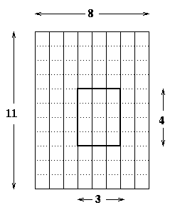
 loc(B(i,j)) = loc(A(5,4)) + (i-1) + (j-1)*LDA

Yet more information is needed by the PBLAS to represent (an arbitrary submatrix) of a 2D block cyclic matrix spread out over an PROW-by-PCOL grid of processors. Indeed, each matrix has a 9-element descriptor containing

1. TYPE (2D block cylic or 1D)
2. Number of rows M
3. Number of column N
4. Row block size MB
5. Column block size NB
6. Processor row 0 <= RSRC < PROW in which A(1,1) lies
7. Processor column 0 <= CSRC < PCOL in which A(1,1) lies
8. BLACS context
9. Leading dimension LDA of local matrix containing A

To refer to a submatrix of such a matrix, we separately need the indices I and J of its upper left corner A(I,J), the number of its rows, and the number of its columns.

For details on the design of the PBLAS, see

Getting software and reports with the WWW