                            d^2 u(x,y)   d^2 u(x,y)
       2D-Laplacian(u)  =   ---------- + ----------  = f(x,y)   for (x,y) in a region Omega
                              d x^2          d y^2
where Omega is a region in the (x,y) plane, say the unit square 0 < x,y < 1.
To make the solution well defined, we also need to specify boundary conditions,
i.e. the value of u(x,y) on the boundary of Omega. We will consider the
simple case
u(x,y) = 0 if (x,y) is on the boundary of Omega
This equation describes the steady-state temperature of a uniform square plate
with the boundaries held at temperature u=0, and f(x,y) equaling the external
heat supplied at (x,y).
In 3 dimensions, the equation is quite similar,
                           d^2 u(x,y,z)   d^2 u(x,y,z)   d^2 u(x,y,z)
       3D-Laplacian(u)  =  ------------ + ------------ + ------------  = f(x,y,z) for (x,y,z) in Omega
                              d x^2           d y^2          d z^2
where Omega is a region in (x,y,z) space. Boundary conditions are also needed,
i.e. the value of u specified on the boundary of Omega.
For simplicity of presentation, we will discuss only the solution of Poisson's equation in 2D; the 3D case is analogous.
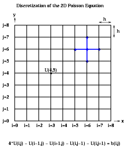
Recalling Lecture 17 again, we discretize this equation by using finite differences: We use an (n+1)-by-(n+1) grid on Omega = the unit square, where h=1/(n+1) is the grid spacing. We let U(i,j) be the approximate solution at x=i*h and y=j*h. This is shown below for n=7, including the system of linear equations it leads to:

The above linear equation relating U(i,j) and the value at its neighbors (indicated by the blue stencil) must hold for 1 <= i,j <= n, giving us N=n^2 equations in N unknowns. When (i,j) is adjacent to a boundary (i=1 or j=1 or i=n or j=n), one or more of the U(i+-1, j+-1) values is on the boundary and therefore 0. b(i,j) = -f(i*h,j*h)*h^2, the scaled value of the right-hand-side function f(x,y) at the corresponding grid point (i,j).
To write this as a linear system in the more standard form P*Uhat = bhat, where Uhat and bhat are column vectors, we need to choose a linear ordering of the unknowns U(i,j). For example, the natural row ordering shown below
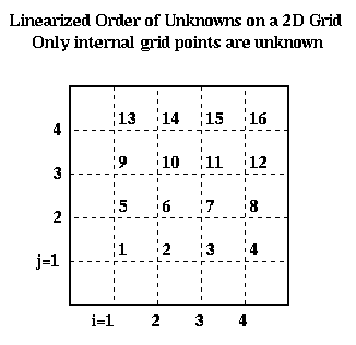
leads to the linear system P*Uhat = bhat:
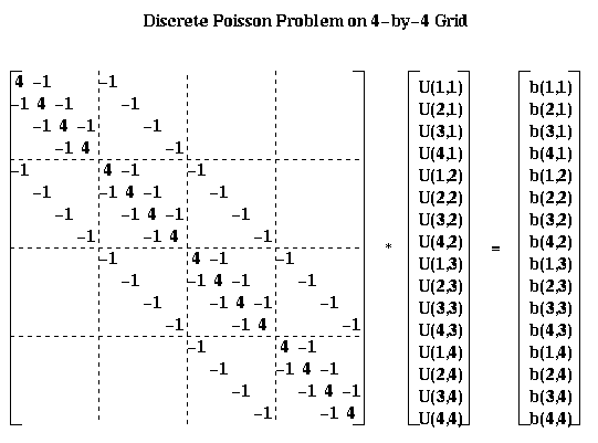
For the most part, we will describe our algorithms in term of the square array U(i,j) rather than the column vector Uhat. But for analysis it is convenient to be able to describe the algorithms using both formulations.
The first column in the table identifies the algorithm, except the last entry, which gives a simple Lower Bound on the running time for any algorithm. The Lower Bound is obtained as follows. For the serial time, the time required simply to print each of the N solution components is N. For the PRAM time, which assumes as many processors as we like and assumes communication is free, we note that the inverse inv(P) of the discrete Poisson matrix P is dense, so that each component of the solution Uhat = inv(P)*bhat is a nontrivial function of each of the N components of bhat. The time required to compute any nontrivial function of N values in parallel is log N.
The second column says whether the algorithm is of Type D=Direct, which means that after a finite number of steps it produces the exact answer (modulo roundoff error), or of Type I=Indirect, which means that one step of the algorithm decreases the error by a constant factor rho<1, where rho depends on the algorithm and N. This means that if one wants the final error to be epsilon times smaller than the initial error, one must take m steps where rho^m <= epsilon. To compute the complexities in the table, we choose m so that rho^m is about as small as the discretization error , i.e. the difference between the true solution x(i*h,j*h) and the exact discrete solution U(i,j). There is no point in making the error in the computed U(i,j) any smaller than this, since this could only decrease the more significant error measure, the difference between the true solution u(i*h,j*h) and the computed U(i,j), by a factor of 2.
The second and third columns give the running time for the algorithm on a serial machine and a PRAM, respectively. Recall that on a PRAM we can have as many processors as we need (shown in the last column), and communication is free. Thus, the PRAM time is a lower bound for any implementation on a real parallel machine. Finally, the fifth column indicated how much storage is needed. LU decomposition requires significantly more storage than the other methods, which require just a constant amount of storage per grid point.
   Algorithm   Type  Serial Time     PRAM Time      Storage  #Procs
   ---------   ----  -----------     ---------      -------  ------
   Dense LU      D       N^3              N           N^2      N^2
   Band LU       D       N^2              N         N^(3/2)     N
   Inv(P)*bhat   D       N^2            log N         N^2      N^2
   Jacobi        I       N^2              N            N        N
   Sparse LU     D       N^(3/2)        N^(1/2)     N*log N     N
   CG            I       N^(3/2)      N^(1/2)*log N    N        N
   SOR           I       N^(3/2)      N^(1/2)          N        N
   FFT           D       N*log N        log N          N        N
   Multigrid     I       N              (log N)^2      N        N
   Lower Bound           N              log N          N
We include methods like dense LU (Gaussian Elimination) even though these are much slower than the fastest methods, because these slower methods solve much more general linear systems than the much faster but more specialized algorithms like Multigrid. This table illustrates that there is often an enormous payoff for using an algorithm specially tuned for the system at hand. Band LU is Gaussian Elimination specialized to take advantage of the fact that none of the zero entries of P more than n entries away from the diagonal ever "fill-in" during Gaussian Elimination, so we can avoid both storing them and doing arithmetic with them. Sparse LU exploits the fact that many other entries in the L and U factors of P are zero, and avoids both computing with or storing any zero entries; this requires interesting linked data structures we will discuss later. Inv(P)*bhat means precomputing and storing the exact N-by-N inverse of P (so we do not count the cost of this precomputation in the complexity), and then doing a matrix-vector multiplication. On a serial machine, this is no faster than any of the subsequent methods, and uses much more storage.
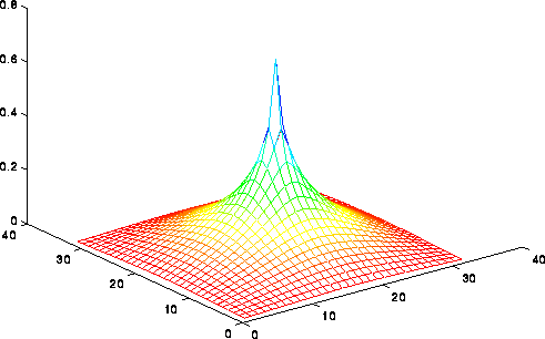
Jacobi, SOR (Successive OverRelaxation) and CG (Conjugate Gradients) can be thought of as performing most nearest neighbor operations on the grid (CG requires summing across the grid too). In other words, information at one grid point can only propagate to an adjacent grid point in 1 iteration. Since the solution U(i,j) at each grid point depends on the value of b(l,m) at every other grid point, it take n steps for information to propagate all the way across the grid. Therefore, we cannot expect a good solution in many fewer than n=sqrt(N) steps, which is what these methods require. This is made more precise by the following picture, which shows the solution of the Poisson equation when b is zero expect for the value 1 in the center. The solution decays logarithmically from the center. If the solution could propagate only from grid point to grid point starting from 0 initial values, then after m < < n steps, one would still have a zero solution outside distance m from the center, even though the solution is large there; this means the error is large, and convergence is impossible.
FFT (the Fast Fourier Transform) and Multigrid can be faster because they move information across the grid in larger steps than merely between neighbors. It is interesting that Multigrid is asymptotically the fastest on a serial machine, attaining the lower bound of N steps. In contrast, FFT is fastest on a PRAM, attaining a lower bound of log N steps. One of our goals in the next two lectures is to do more detailed performance modeling of these methods, taking communication costs into account, to see which one we expect to be fastest in practice.
U(i,j) = (U(i-1,j) + U(i+1,j) + U(i,j-1) + U(i,j+1) + b(i,j))/4
We let U(i,j,m) be our approximation for U(i,j) after the m-th iteration.
We can use any initial guess U(i,j,0); U(i,j,0)=0 will do. To get a
formula for U(i,j,m+1) in terms of the previous iteration U(i,j,m), we
simply use
U(i,j,m+1) = (U(i-1,j,m) + U(i+1,j,m) + U(i,j-1,m) + U(i,j+1,m) + b(i,j))/4
In other words, U(i,j,m+1) is just a weighted average of its four
neighboring values and b(i,j).
We analyze the convergence rate of Jacobi as follows. We present only the final results; for details, see any good text on numerical linear algebra, such as "Lecture Notes on Numerical Linear Algebra", J. Demmel, Berkeley Lecture Notes in Mathematics, Mathematics Dept, UC Berkeley (coming next semester to a URL near you). To state the result we define the error as the root-sum-of-squares of the error at each grid point:
error(m) = sqrt( sum_{ij} ( U(i,j,m) - U(i,j) )^2 )
It turns out that Jacobi decreases the error by a constant factor
rho_Jacobi(n) < 1 depending on dimension at each step:
   error(m) <= rho_Jacobi(n) * error(m-1)
            <= ( rho_Jacobi(n) )^m * error(0)
where
rho_Jacobi(n) = cos(pi/(n+1))When n is large, the interesting case, we can approximate rho_Jacobi(n) by
rho_Jacobi(n) ~ 1 - .5*(pi/(n+1))^2which gets closer to 1 as n grows. So to decrease the error by a factor of 2, say, requires taking m iterations where
      .5 > ( rho_Jacobi(n) )^m
         ~ ( 1 - .5*(pi/(n+1))^2 )^m
         ~ 1 - .5*(pi/(n+1))^2 * m         ... when n is large
or
m ~ ((n+1)/pi)^2
In other words, convergence gets slower
for large problems, with the number of steps proportional to N = n^2.
This make the serial complexity
    Serial complexity of Jacobi = number_of_steps * cost_per_step
                                = O(N) * O(N)
                                = O(N^2)
This is easy to implement in parallel, because each grid cell value may
be updated independently. On a PRAM, this means the cost per step
is O(1), lowering the PRAM complexity to O(N).
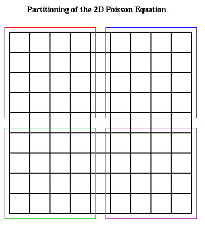
On a realistic parallel machine, one would simply assign grid point (i,j)
to processors in a block fashion as shown below, and have each processor
update the values of U(i,j,m+1) at the grid point it owns. This requires U
values on the boundary of the blocks to be communicated to neighboring
processors. When n >> p, so that each processor owns a large number n^2/p
of grid points, the amount of data communicated, n/p words with each neighbor,
will be relatively small.
To express the parallel running time in detail, we let
     p = number of processors
     f = time per flop
     alpha = startup for a message
     beta = time per word in a message
Then
     Time(Jacobi) = number_of_steps * cost_per_step
                  = O(N) * ( (N/p)*f + alpha + (n/p)*beta )
                         ... O(N/p) flops to update local values
                         ... alpha for the start up of messages to each neighbor
                         ... O(n/p) boundary value communicated to neighbors
                  = O(N^2/p)*f + O(N)*alpha + O(N^(3/2) /p)*beta
Later we will compare this expression to similar expressions for other methods.
The phenomenon of convergence slowing down, and needing to take more steps for large problems, is a common phenomenon for many methods and problems. It is not true for Multigrid, however, which takes a constant number of iterations to decrease the error by a constant factor, and so makes it very attractive.
The first improvement is motivated by examining the serial implementation, and noticing that while evaluating
U(i,j,m+1) = (U(i-1,j,m) + U(i+1,j,m) + U(i,j-1,m) + U(i,j+1,m) + b(i,j))/4
new values for the solution at some of the grid points on the right hand side
are already available, and may be used. This leads to the algorithm
     U(i,j,m+1) = (U(i-1,j,latest) + U(i+1,j,latest) +
                   U(i,j-1,latest) + U(i,j+1,latest) + b(i,j) )/4
where "latest" is either m or m+1, depending on whether that particular
grid point has been updated already. This depends on the order in which
we loop through the (i,j) pairs. For example, if we use the same rowwise
ordering as in an earlier figure, we get the so-called Gauss-Seidel
algorithm:
       for i=1 to n
           for j=1 to n
               U(i,j,m+1) = (U(i-1,j,m+1) + U(i+1,j,m) +
                             U(i,j-1,m+1) + U(i,j+1,m) + b(i,j) )/4
           end for
       end for
This particular update order cannot be straightforwardly parallelized,
because there is a recurrence, with each U(i,j,m+1) depending on the
immediately previously updated value U(i-1,j,m+1).
So instead we loop through the grid points in the Red-Black order (named after the resemblance to a chess board) shown below.
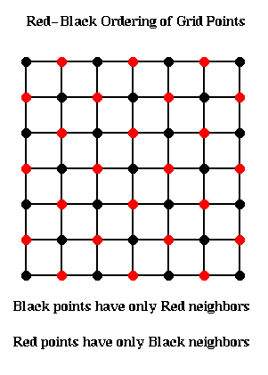
The idea is to update all the black points, followed by all the red points. The black grid points are connected only to red grid points, and so can all be updated simultaneously using the most recent red values. Then the red values can be updated using the most recent black values. This yields the following algorithm:
     for all black (i,j) grid points
         U(i,j,m+1) = (U(i-1,j,m) + U(i+1,j,m) +
                       U(i,j-1,m) + U(i,j+1,m) + b(i,j))/4
     end for
     for all red (i,j) grid points
         U(i,j,m+1) = (U(i-1,j,m+1) + U(i+1,j,m+1) +
                       U(i,j-1,m+1) + U(i,j+1,m+1) + b(i,j))/4
     end for
This can implemented in two parallel steps, one for updating the red points,
and one for the black.
By itself, this idea does not accelerate convergence. It turns out to converge twice as fast (rho_Gauss_Seidel(n) = rho_Jacobi(n)^2), but on a PRAM each parallel Gauss-Seidel step takes the same time as two parallel Jacobi steps, so there is no overall benefit.
The second improvement is called Successive Overrelaxation, and depends on the Red-Black ordering for its speedup. Let us rewrite the algorithm so far as
     U(i,j,m+1) = some_expression
                      ... an abbreviation for the update scheme above
                = U(i,j,m) + (some_expression - U(i,j,m))
                = U(i,j,m) + correction(i,j,m)
The idea behind overrelaxation is that if correction(i,j,m) is a
good direction in which to move U(i,j,m) to make it a better solution,
one should move even farther in that direction, by a factor w>1:
U(i,j,m+1) = U(i,j,m) + w * correction(i,j,m)
w is called the overrelaxation factor (w<1 would correspond to underrelaxation,
which is not worth doing). The word successive refers to using the latest
data to evaluate the correction.
Altogether, the SOR(w) algorithm is as follows:
     for all black (i,j) grid points
         U(i,j,m+1) = U(i,j,m) +
                      w * (U(i-1,j,m) + U(i+1,j,m) +
                           U(i,j-1,m) + U(i,j+1,m) + b(i,j) - 4*U(i,j,m))/4
     end for
     for all red (i,j) grid points
         U(i,j,m+1) = U(i,j,m) +
                      w * (U(i-1,j,m+1) + U(i+1,j,m+1) +
                           U(i,j-1,m+1) + U(i,j+1,m+1) + b(i,j) - 4*U(i,j,m))/4
     end for
As before, we measure the error of iteration m by
error(m) = sqrt( sum_{ij} ( U(i,j,m) - U(i,j) )^2 )
As with Jacobi, SOR(w) decreases the error by a constant factor
rho_SOR(n,w) < 1 at each step:
   error(m) <= rho_SOR(n,w) * error(m-1)
            <= ( rho_SOR(n,w) )^m * error(0)
We want to pick w to minimize rho_SOR(n,w). There turns out to be a simple
expression for the minimizing w,
w_opt = 2 / ( 1 + sin(pi/(n+1)) )
which is between 1 and 2. The corresponding rho_SOR(n,w_opt) is
rho_SOR(n,w_opt) = ( cos(pi/(n+1)) / ( 1 + sin(pi/(n+1)) ) )^2
As with Jacobi, rho_SOR(n,w_opt) approaches 1 as n grows, so that
convergence slows down, but it slows down much less than for Jacobi:
rho_SOR(n,w_opt) ~ 1 - 2*pi/(n+1)
Therefore, reducing the error by a factor of 2, say,
requires taking m iterations where
      .5 > ( rho_SOR(n,w_opt) )^m
         ~ ( 1 - 2*pi/(n+1) )^m
         ~ 1 - 2*pi/(n+1) * m         ... when n is large
or
m ~ (n+1)/(2*pi)
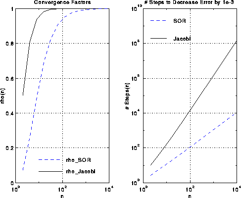
This is approximately the square root of the number of steps Jacobi requires.
This is shown in the figures below.
A complexity analysis similar to that for Jacobi shows that
     Time(SOR) = number_of_steps * cost_per_step
               = O(sqrt(N)) * ( (N/p)*f + alpha + (n/p)*beta )
                         ... O(N/p) flops to update local values
                         ... alpha for the start up of messages to each neighbor
                         ... O(n/p) boundary value communicated to neighbors
               = O(N^(3/2) /p)*f + O(sqrt(N))*alpha + O(N /p)*beta
     x = initial guess for inv(A)*b
     r = b - A*x
     p = r
     repeat
        v = A*p                           ... matrix-vector multiply
        a = ( r'*r ) / ( p'*v )           ... dot product (BLAS1)
        x = x + a*p                       ... saxpy (BLAS1)
        new_r = new_r - a*v               ... saxpy
        b = ( new_r'*new_r ) / ( r'*r )   ... dot product
        p = new_r + b*p                   ... saxpy
        r = new_r
     until ( new_r'*new_r small enough )
We are going to rewrite the discrete Poisson equation as a slightly different matrix equation. To motivate it, consider the continuous Poisson equation
          d^2 u(x,y)   d^2 u(x,y)
          ---------- + ----------  = f(x,y)
            d x^2          d y^2
and discretize one derivative term at a time.
Then
          d^2 u(i*h,j*h)   U(i-1,j) - 2*U(i,j) + U(i+1,j)
          -------------- ~ ------------------------------
               d x^2                   h^2
Now consider the n-by-n matrix whose (i,j) entry is the right-hand-side of
the above equation. We claim that this matrix may be written as the
matrix-matrix product (-1/h^2)*T*U, where U is the n-by-n matrix of U(i,j)'s,
and T is the familiar symmetric tridiagonal matrix
              [  2  -1                 ]
              [ -1   2  -1             ]
          T = [     -1   2  -1         ]
              [       ... ... ...      ]
              [             -1  2  -1  ]
              [                -1   2  ]
A formal proof requires the simple computation:
       (T*U)(i,j) = sum_k T(i,k)*U(k,j)
                  =  T(i,i-1)*U(i-1,j) +   T(i,i)*U(i,j) + T(i,i+1)*U(i+1,j)
                          ... since only 3 entries of row i of T are nonzero
                  = -U(i-1,j) + 2*U(i,j) - U(i+1,j)
A completely analogous argument shows that
          d^2 u(i*h,j*h)   U(i-1,j) - 2*U(i,j) + U(i+1,j)   -1
          -------------- ~ ------------------------------ = --- * (U*T)(i,j)
               d x^2                   h^2                  h^2
and so the Discrete Poisson equation may be written
T*U + U*T = B
where the (i,j)-th entry of B is b(i,j), as before.
Now recall that in Lecture 20, we had an explicit expression for the eigenvalues and eigenvectors of T: T = Q*Lambda*Q' where Lambda is a diagonal matrix of eigenvalues
Lambda(j,j) = 2*(1-cos(j*pi/(n+1))
and Q is an orthogonal matrix whose columns are eigenvectors:
Q(j,k) = sin(j*k*pi/(n+1)) * sqrt(2/(n+1)) = Q(k,j)
Now plug T = Q*Lambda*Q' into T*U+U*T=B to get
(Q*Lambda*Q')*U + U*(Q*Lambda*Q') = B
Premultiply this equation by Q' ( = inverse(Q)) and postmultiply it by Q to get
Lambda*(Q'*U*Q) + (Q'*U*Q)*Lambda = Q'*B*Q
or
Lambda*(Ubar) + (Ubar)*Lambda = Bbar
where we have defined Ubar=Q'*U*Q and Bbar=B'*B*Q.
The (j,k)-th entry of this last equation is simple to compute,
since Lambda is diagonal:
Lambda(j,j)*Ubar(j,k) + Ubar(j,k)*Lambda(k,k) = Bbar(j,k)
which we may solve for Ubar(j,k) as follows:
Ubar(j,k) = Bbar(j,k)/(Lambda(j,j)+Lambda(k,k))
This lets us state the overall high-level algorithm:
  (1) Compute Bbar = Q'*B*Q
  (2) Compute Ubar(j,k) = Bbar(j,k)/(Lambda(j,j)+Lambda(k,k)) for each j,k
  (3) Compute U = Q*Ubar*Q'
Step 2 is embarrassingly parallel, costing n^2 divisions by precomputable constants Lambda(j,j)+Lambda(k,k). Steps 1 and 3 require four matrix-matrix multiplications by Q=Q'. If we did this using a conventional matrix multiplication requiring 2*n^3 operations, the whole algorithm would take about 8*n^3 = 8*N^(3/2) operations, no faster than SOR.
It turns out that a multiplying a vector v by Q can be done in O(n log n) time using the FFT. This reduces the cost of Steps 1 and 3 of the algorithm to O(n^2 log n) = O(N log N), since matrix-matrix multiplication Q*B requires n matrix-vector multiplies, one for each column of B. To see this requires a brief review of the FFT
Definition. The Discrete Fourier Transform of an m-by-1 vector v is the matrix-vector product F*v, where F is an m-by-m matrix defined as follows. Let omega = exp(2*pi*i/m) = cos(2*pi/m) + i*sin(2*pi/m), i.e. a complex number with absolute value 1, whose m-th power is 1 (an m-th root of unity). Then for 0 <= j,k <= m-1, F(j,k) = omega^(j*k).
A standard fact about F is that inv(F) = complex_conjugate(F)/m, so that F/sqrt(m) is a unitary matrix (the complex equivalent of an orthogonal matrix). This means that multiplying by F and inverse(F) are essentially equivalent problems.
The Fast Fourier Transform (FFT) is an algorithm to compute the Discrete Fourier Transform F*v in O(m log m) time instead of O(m^2) time.
     F(j,k) = cos(2*pi*j*k/(2*(n+1))) + i * sin(2*pi*j*k/(2*(n+1)))
            = cos(pi*j*k/(n+1) + i * sin(pi*j*k/(n+1))
By comparing this expression with the expression for Q, we see that
Q is a submatrix of F:
Q = Imag( F(1:n, 1:n) )
where Imag(x) is the imaginary part of x.
Thus, one can write
Q*v = Imag( (F*[0;v;zeros(n,1)]) (1:n) )
In other words, we could extend v with one 0 at the top and n zeros at the
bottom, do a 2*(n+1) point FFT, and extract the imaginary part of
components 1 through n from components 0 through 2*n+1. Matlab code
for a function fast_sine_transform(v) which performs Q*V is as follows
(note that it uses Matlab's built-in fft function).
     % Fast Sine Transform on input matrix V of dimension n-by-m
     function Y=fast_sine_transform(V)
     [n,m]=size(V);
     V1=[zeros(1,m);V;zeros(n+1,m)];
     V2=imag(fft(V1));
     % In Matlab vectors and matrices are indexed starting at 1, not 0
     Y=V2(2:n+1,:);
Using fast_sine_transform, a Matlab implementation of the entire FFT-based Poisson solver is
    % Solve the discrete Poisson equation on an n-by-n grid with right hand side b
    function X=Poisson_FFT(B)
    [n,m]=size(b);
    % Form eigenvalues of matrix T(nxn)
    L=2*(1-cos((1:n)*pi/(n+1)));
    % Form reciprocal sums of eigenvalues
    % Include scale factor 2/(n+1)
    LL=(2/(n+1))*ones(n,n)./(L'*ones(1,n)+ones(n,1)*L);
    % Solve, using the Fast Sine Transform
    X = fast_sine_transform(b');
    X = fast_sine_transform(X');
    X = LL.*X;
    X = fast_sine_transform(X');
    X = fast_sine_transform(X');
We begin by showing how to interpret the product F*v as polynomial evaluation of the polynomial
V(x) = sum_{k=0}^{m-1} x^k * v(k)
at the points x = omega^0, omega^1, omega^2, ..., omega^(m-1):
     (F*v)(j) = sum_{k=0}^{m-1} F(j,k) * v(k)
              = sum_{k=0}^{m-1} omega^(j*k) * v(k)
              = sum_{k=0}^{m-1} (omega^j)^k * v(k)
              = V(omega^j)
Conversely, one can interpret multiplication by inv(F) as
polynomial interpolation, i.e. computing the coefficients of
a polynomial given its value at m points omega^j.
Now break up the polynomial V(x) into two parts, those consisting of even powers of x, and those consisting of odd powers of x:
      V(x) = v(0) + omega^2 * v(2) + omega^4 * v(4) + ...
                  + omega^1 * v(1) + omega^3 * v(3) + ...
           = (v(0) + omega^2 * v(2) + omega^4 * v(4) + ...)
             + x * (v(1) + omega^2 * v(3) + omega^3 * v(5) + ...)
(*)        = V_even(x^2) + x * V_odd(x^2)
Since V is a polynomial of degree m-1, V_even and V_odd are polynomials
of degree m/2 - 1, which we need to evaluate at the points
(omega^j)^2, for 0 <= j <= m-1. But this is really just (m/2) different
points omega^(2*j) for 0 <= j <= (m/2)-1 since
    (omega^(j+m/2))^2 = (omega^j * omega^(m/2))^2
                      = (omega^j)^2 * omega^m
                      = (omega^j)^2       ... since omega^m = 1 by construction
Thus, evaluating V(x) at m values omega^j is equivalent to evaluating
two half sized problems (V_odd and V_even at half as many points),
and then combining their values in a simple way. This leads to the
following recursive, divide-and-conquer algorithm for the FFT:
     function x = FFT(v,omega,m)
         if m=1 then
              return v(0)
         else
            v_even = FFT(v(0:2:m-2), omega^2, m/2)
                     ... v(0:2:m-2) = v(0,2,4,...,m-2)
            v_odd  = FFT(v(1:2:m-1), omega^2, m/2)
                     ... v(1:2:m-1) = v(1,3,5,...,m-1)
            omegav = [ omega^0, omega^1, omega^2, ... , omega^((m/2)-1) ]
                     ... in practice these coefficients are precomputed
                     ... and stored in a table
            return x = [v_even + ( omegav .* v_odd ),
                        v_even - ( omegav .* v_odd )]
                     ...  omegav .* v_odd is the component-wise product of these two vectors
         end if
The reason for using +omegav.*v_odd and -omegav.*v_odd is that when
x = omega^(j+(m/2)) in equation (*) above,
omega^(j+(m/2)) = omega^j * omega^(m/2) = -omega*j
We compute the complexity of this algorithm as follows. Let FFT_time(m) be the cost of the algorithm on an input of size m. Then from the structure of the algorithm
     FFT_time(m) = 2 * FFT_time(m/2)  ... for the two recursive calls
                   + O(m)             ... for the m/2 products, sums, and
                                      ... differences in computing x
Change variables to s = log_2 m to get
FFT_time(s) = 2 * FFT_time(s-1) + O(2^s)
This simple recurrence has the value FFT_time(s) = O(2^s) + O(2^s) + ... O(2^s) (s terms), or O(s*2^s) = O(m log m), as desired.
It is not necessary for m to be a power of 2 to use the divide-and-conquer technique in this algorithm. Indeed, Gauss first invented this algorithm for m=12 centuries ago. To be efficient, m should be a product of many small prime factors.
k = k(0)k(1)...k(s-2)k(s-1)_2
of the output vector contains component
reverse(k) = k(s-1)k(s-2)...k(2)k(0)_2
of F*v.
     for j = 0 to s-1              ... for each level of the call tree
                                   ... from bottom to top
         for  k = 0 to (m/2)-1     ... for each vector entry
              t0 = v[k(0)k(1)...k(j-1)0k(j)...k(s-2)]
                                   ... the subscript is equal to k with
                                   ... bit j set to 0
              t1 = v[k(0)k(1)...k(j-1)1k(j)...k(s-2)]
                                   ... the subscript is equal to k with
                                   ... bit j set to 1
              w = omega^[0k(j-1)...k(0)0...0]
                                   ... a power of omega stored in a table
              x = w*t1
              v[k(0)k(1)...k(j-1)0k(j)...k(s-2)] = t0 + x
                                   ... update location of v containing t0
              v[k(0)k(1)...k(j-1)1k(j)...k(s-2)] = t0 - x
                                   ... update location of v containing t1
         end for
     end for
The algorithm corresponds to the recursive version because setting the
j-th bit of a subscript to 0 is equivalent to taking the even subset of
subscripts, and setting the j-th bit to 1 is equivalent to taking the
odd subset.
     When j=0            When j=1           When j=2           When j=3
       When k=0            When k=0           When k=0           When k=0
          t0 = v[0000]       t0 = v[0000]       t0 = v[0000]       t0 = v[0000]
          t1 = v[1000]       t1 = v[0100]       t1 = v[0010]       t1 = v[0001]
       When k=1            When k=1           When k=1           When k=1
          t0 = v[0001]       t0 = v[0001]       t0 = v[0001]       t0 = v[0010]
          t1 = v[1001]       t1 = v[0101]       t1 = v[0011]       t1 = v[0011]
       When k=2            When k=2           When k=2           When k=2
          t0 = v[0010]       t0 = v[0010]       t0 = v[0100]       t0 = v[0100]
          t1 = v[1010]       t1 = v[0110]       t1 = v[0110]       t1 = v[0101]
       When k=3            When k=3           When k=3           When k=3
          t0 = v[0011]       t0 = v[0011]       t0 = v[0101]       t0 = v[0110]
          t1 = v[1011]       t1 = v[0111]       t1 = v[0111]       t1 = v[0111]
       When k=4            When k=4           When k=4           When k=4
          t0 = v[0100]       t0 = v[1000]       t0 = v[1000]       t0 = v[1000]
          t1 = v[1100]       t1 = v[1100]       t1 = v[1010]       t1 = v[1001]
       When k=5            When k=5           When k=5           When k=5
          t0 = v[0101]       t0 = v[1001]       t0 = v[1001]       t0 = v[1010]
          t1 = v[1101]       t1 = v[1101]       t1 = v[1011]       t1 = v[1011]
       When k=6            When k=6           When k=6           When k=6
          t0 = v[0110]       t0 = v[1010]       t0 = v[1100]       t0 = v[1100]
          t1 = v[1110]       t1 = v[1110]       t1 = v[1110]       t1 = v[1101]
       When k=7            When k=7           When k=7           When k=7
          t0 = v[0111]       t0 = v[1011]       t0 = v[1101]       t0 = v[1110]
          t1 = v[1111]       t1 = v[1111]       t1 = v[1111]       t1 = v[1111]
We may represent this graphically, with an m-by-(s+1) (16-by-5) grid of points.
Each column of m points represents the values in the array v at some stage
in the computation. The leftmost column, column 0, represents the original
data. The next column, column 1, represents the data after the computations
performed when j=0,
the next column represents the data after j=1, and so on, until the
rightmost column represents the final data.
There is an edge from a grid point v0 in column j to a grid point v1 in column j+1, if the data at v1 depends on the data at v0. From examining the algorithm, we see that there is an edge from both grid points
     [k(0)k(1)...k(j-1)0k(j)...k(s-2)]  and
     [k(0)k(1)...k(j-1)1k(j)...k(s-2)]  in column j
to the same grid points points in column j+1, for a total of 4 edges
connecting this pair of points.
These 4 edges form what looks like a "butterfly" in the figure below,
where we have color-coded the edges so that edges corresponding to the
same butterfly connecting adjacent columns have the same color.
Here is the graph in the case m=16. The first column of butterflies
connects grid points whose numbers differ in bit 0 (the leftmost bit).
For example, the black butterfly connects 0000 and 1000. The second
column of butterflies connects grid points whose numbers differ in bit 1;
for example the black butterfly connects 0000 and 0100.
The next black butterfly connect 0000 and 0010, and the rightmost black
butterfly connects 0000 and 0001.
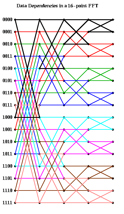
This analysis is enough to compute the PRAM complexity of the FFT: Each of the s rightmost columns can be computed in one time step using m processors, for a complexity of O(s) = O(log m).
For a real parallel implementation, we need to take communication costs into account, and this is dictated by our choice of layout: which processors own which entries of the vector v. The following discussion may be found in "LogP: Towards a realistic model of parallel computation, Culler, Karp, Patterson et al, which is in the class reader, or the textbook.
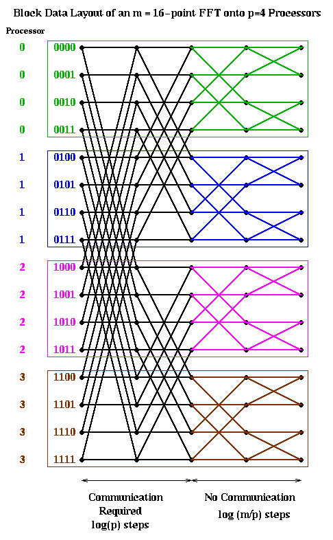
Let us consider two obvious candidates which we considered before in the case of Gaussian elimination: blocked and cyclic. The block case is shown below, with m=16 and p=4. The processor numbers are color coded. Edges which cross processor boundaries, and so require communication, are black. Edges within a processor, which require no communication, are color coded by the local processor color. In the block case, note that the leading log(p) bits of an address determine the processor (green is processor 00, blue is 01, magenta is 10, and brown is 11). Thus, in general, the first log(p) stages require communication, because addresses of data to be combined differ in their leading log(p) bits. The last log(m/p) stages are local, and require no communication.
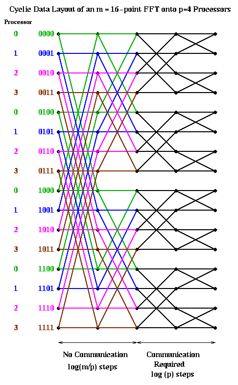
The cyclic case is shown below, color coded in the same way. In this case, the trailing log(p) bits of an address determine the processor. Therefore, the last log(p) stages require communication, and the first log(m/p) stages are local.
Let us analyze the parallel complexity of these algorithms. As before we use the parameters.
     p = number of processors
     f = time per flop
     alpha = startup for a message
     beta = time per word in a message
Then both the block and cyclic implementations require
     Time(block FFT) = Time(cylic FFT) =
            2*m*log(m)/p * f       ... 2*m/p flops at log(m) stages
           + log(m/p) * alpha      ... one message per processor per stage
                                   ... for log(m/p) stages
           + m*log(m/p)/p * beta   ... m/p words per message
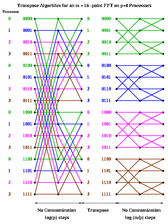
An alternative implementation is start with a cyclic implementation, and then transpose the data to have a block layout after the first log(p) steps. This way the first log(p) stages require no communication, then a transpose (a significant amount of communication) is performed, and finally the last log(m/p) stages are again local. (This assumes m>=p^2, which we now assume, since we expect many more points than processors. Otherwise, there may be more transposes required.) This is shown below.
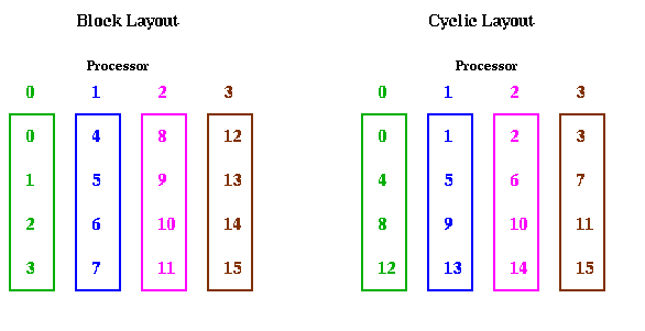
The reason we call converting from cyclic to block layout (or back) transposing is shown below for m=16 and p=4. When the data layout is seen in this way, it clearly looks like transposing a matrix.
The cost of this algorithm is
     Time(transpose FFT) =
          = 2*m*log(m)/p * f       ... 2*m/p flops at log(m) stages
           + (p-1) * alpha         ... p-1 messages per processor to transpose
           + m*(p-1)/p^2 * beta    ... m/p^2 words per message
Computing Time(transpose FFT) with Time(block FFT) or Time(cyclic FFT),
we see that the transpose FFT sends less data overall, but has more messages.
Thus, one expects the transpose to do well in a low latency, high bandwidth
environment, and the block or cyclic to do well in a high latency,
low bandwidth environment.
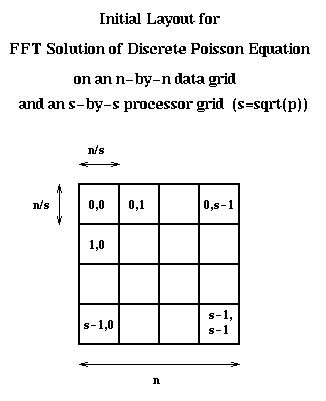
The algorithm is now easy to describe. Each of the four multiplications by Q (FFTs) is analogous. In the first multiplication Q*B, each processor column of s processors cooperates to perform n/s FFTs. This costs
     Time(Q*B) =
          O((n*log(n)/s) * (n/s) * f   ... O(n*log(n)/s flops per FFT
                                       ... times n/s FFTs
           + (s-1) * alpha             ... s-1 messages per processor to transpose
           + n^2*(s-1)/s^3 * beta      ... (n/s^2)*(n/s) words per message
       = O(N*log N / p)*f + (s-1)*alpha + N*((s-1)/s)/p *beta
Each of the four pre- or postmultiplications by Q costs the same (for
premultiplications, processor columns cooperate, and for postmultiplications,
processor rows cooperate). Finally the local divisions by
Lambda(j,j)+Lambda(k,k) costs n^2/p flops, which is a lower order term
compared to the flops in the multiplications by Q.
The total cost is therefore about 4*Time(Q*B) shown above.