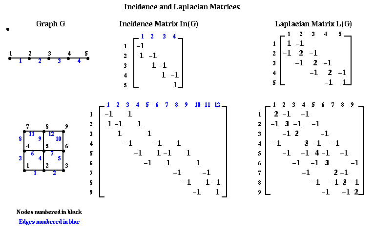
We will first describe the algorithm, and then give three related justifications for its efficacy. Let G=(N,E) be an undirected, unweighted graph without self edges (i,i) or multiple edges from one node to another. We define two matrices related to this graph.
Definition The incidence matrix In(G) of G is an |N|-by-|E| matrix, with one row for each node and one column for each edge. Suppose edge e=(i,j). Then column e of In(G) is zero except for the the i-th and j-th entries, which are +1 and -1, respectively.
Note that there is some ambiguity in this definition, since G is undirected; writing edge e=(i,j) instead of (j,i) is equivalent to multiplying column e of In(G) by -1. We will see that this ambiguity will not be important to us.
Definition The Laplacian matrix L(G) of G is an |N|-by-|N| symmetric matrix, with one row and column for each node. It is defined as follows.
        (L(G))(i,j) = degree of node i (number of incident edges) if i=j
                    = -1   if i!=j and there is an edge (i,j)
                    =  0   otherwise
Here are some small examples. Note the similarity between the Laplacian graph of the mesh, and the matrix for the discrete Poisson equation, introduced in Lecture 16. With z zero right hand side, we also called this discrete equation Laplace's equation. We will pursue this physical analogy below.

The following theorem state some important facts about In(G) and L(G). It introduces us to the idea that the eigenvalues and eigenvectors of L(G) are related to the connectivity of G.
Theorem 1. Given a graph G, its associated matrices In(G) and L(G) have the following properties.
          lambda = norm(In(G)'*v)^2 / norm(v)^2        where norm(z)^2 = sum_i z(i)^2
                 = sum_{all edges e=(i,j)} (v(i)-v(j))^2  / sum_i v(i)^2
For a proof of this theorem, click here.
Part 6 of Theorem 1 motivates the following definition.
Definition (M. Fiedler, "Algebraic Connectivity of Graphs", Czech. Math. J. 23:298--305, 1973). lambda(2)(L(G)) is called the algebraic connectivity of G.
Now we can state our algorithm for spectral bisection of a graph.
    Compute the eigenvector v(2) corresponding to lambda(2) of L(G)
    for each node n of G
       if v(2)(n) < 0
          put node n in partition N-
       else
          put node n in partition N+
       endif
    endfor
First we show that this partition is at least reasonable, because it tends to give connected components N- and N+:
Theorem 2. (M. Fiedler, "A property of eigenvectors of nonnegative symmetric matrices and its application to graph theory", Czech. Math. J. 25:619--637, 1975.) Let G be connected, and N- and N+ be defined by the above algorithm. Then N- is connected. If no v(2)(n) = 0, N+ is also connected.
For a partial proof, click here.
There are a number of reasons lambda(2) is called the algebraic connectivity. Here is another.
Theorem 3. (Fiedler). Let G=(N,E) be a graph, and G1=(N,E1) a subgraph, i.e. with the same nodes and a subset of the edges, so that G1 is "less connected" than G. Then lambda(2)(L(G1)) <= lambda(2)(L(G)), i.e. the algebraic connectivity of G1 is also less than or equal to the algebraic connectivity of G.
We will prove this later, after we introduce more machinery.

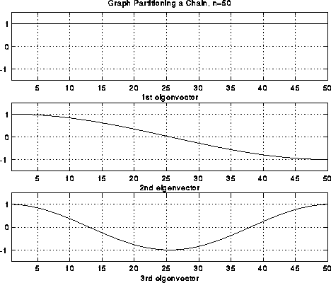
Note that we have also labeled each part of the string as to whether it is above the rest position (+), or below (-). In the case of the second frequency lambda(2), half the string is labeled +, and half is labeled -, effectively bisecting the string into two equal sized, connected components. It turns out that if we build this vibrating string from a finite set of identical masses (nodes) connected by identical springs (edges), write down Newton's Laws of motion for the masses, and solve for the frequencies and shapes of the vibrational modes, we will get precisely the eigenvalues and eigenvectors of the Laplacian L(G) of the graph G, where G consists of a chain of nodes with nearest neighbor connections. Therefore, the second eigenvector of L(G) is the shape of the second mode of vibration, and divide the graph in half.
In the case of more complicated graphs than simple chains, the same intuition applies. It is easiest to understand in the case of planar graphs, which we can think of as a kind of trampoline; again the second mode of vibration divides the graph (trampoline) into two halves.
Let us perform this construction more explicitly in the case of a string. In the figure below, we let x(i) represent the (small) displacement of mass i from the horizontal.
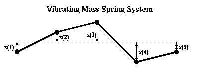
If the displacement is small, the force on mass i is
      force(i) = k*(x(i-1)-x(i)) + k(x(i+1)-x(i))
               = k*(x(i-1) - 2*x(i) + x(i+1))
where k is a spring constant. We assume that the spring from x(i) to x(i+1) is stretched
proportional to the distance x(i+1)-x(i). If this difference is positive, so mass i+1 is
higher than mass i, then the force is upwards, or positive. Newton's law tells us F=ma or
          d^2 x(i)
      m * -------- = force(i) =  k*(x(i-1) - 2*x(i) + x(i+1))
           d t^2
We need to be careful about what happens at the end masses. The simplest, and nearly correct,
decision is to fix x(0)=x(n+1)=0 (like a taut spring). This lets us write down the system of ODEs
           [  x(1) ]                [ 2*x(1)-x(2)           ]        [  2 -1          ]   [  x(1) ]
           [  x(2) ]                [ -x(1)+2*x(2)-x(3)     ]        [ -1 2 -1        ]   [  x(2) ]
  m * d^2  [  .... ] / d t^2 = -k * [      ...              ] = -k * [    ...         ] * [ ....  ]
           [ x(n-1)]                [ -x(n-2)+2*x(n-1)-x(n) ]        [       -1  2 -1 ]   [ x(n-1)]
           [  x(n) ]                [ -x(n-1)+2*x(n)        ]        [          -1  2 ]   [  x(n) ]

                                        [  x(1) ]
                                        [  x(2) ]
                             = -k * M * [  .... ]
                                        [ x(n-1)]
                                        [  x(n) ]
or yet more briefly,
                d^2 x(t)
       -(m/k) * -------- =  M * x(t)
                 d^2 t
where x(t) is a vector [x(1),...,x(n)]'. We seek solutions of the form
x(t) = sin(a*t)*x0, where a and x0 are a scalar and vector to be determined. Plugging in to the
last equation yields
(m/k)*a^2*sin(a*t)*x0 = M * sin(a*t) * x0
Canceling sin(a*t), which is never zero, yields
M * x0 = (m/k)*a^2 * x0 = e * x0
Thus x0 is an eigenvector of M and e=(-m/k)*a^2 is an eigenvalue. We know the eigenvalues and
eigenvector of M explicitly; as can be confirmed by simple trigonometry, the i-th pair is given by
            [ sin(1*i*pi/(n+1))     ]
            [ sin(2*i*pi/(n+1))     ]
       x0 = [ ......                ]     e = 2*(1-cos(i*pi/(n+1)))
            [ sin((n-1)*i*pi/(n+1)) ]
            [ sin(n*i*pi/(n+1))     ]
In other words, we just get sine curves of varying frequencies, exactly matching the curves
pictured above. Furthermore, when n is large and i is small,
(m/k) * a^2 = e = 2*(1-cos(i*pi/(n+1))) ~ ( i*pi/(n+1) )^2
so the frequency of vibration
a ~ sqrt(k/m)*pi/(n+1) * i
In other words, the frequencies of successive modes of vibrations are just multiples of
the base frequency, thus providing the harmonics we expect from a plucked string.
Unfortunately, M is not quite the Laplacian L(G) of the simple graph G of n nodes connected in a chain; the (1,1) and (n,n) entries are 2 instead of 1. To make the analogy between spectral bisection and the vibrating string exact, we need a slightly different mass-spring system. This is shown in the figure below. There are n horizontal rods, and on each rod a mass m can slide back and forth frictionlessly. These identical masses are connected with identical springs as before. x(i) is the horizontal displacement from rest.
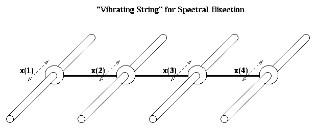
The only difference from before in the equations of motion is for masses 1 and n, the ones at the end. Since they are only tied to one moving mass, rather than one moving mass and one fixed endpoint, we get
          d^2 x(1)
      m * -------- = force(1) =  k*(x(2) - x(1))
           d t^2
and
          d^2 x(n)
      m * -------- = force(1) =  k*(x(n-1) - x(n))
           d t^2
which leads to
           [  x(1) ]                [ x(1)-x(2)             ]        [  1 -1          ]   [  x(1) ]
           [  x(2) ]                [ -x(1)+2*x(2)-x(3)     ]        [ -1 2 -1        ]   [  x(2) ]
  m * d^2  [  .... ] / d t^2 = -k * [      ...              ] = -k * [    ...         ] * [ ....  ]
           [ x(n-1)]                [ -x(n-2)+2*x(n-1)-x(n) ]        [       -1  2 -1 ]   [ x(n-1)]
           [  x(n) ]                [ -x(n-1)+x(n)          ]        [          -1  1 ]   [  x(n) ]

                                           [  x(1) ]
                                           [  x(2) ]
                             = -k * L(G) * [  .... ]
                                           [ x(n-1)]
                                           [  x(n) ]
One can again confirm by simple trigonometry, that the i-th eigenvalue and eigenvector of L(G) are
given by
            [ cos((0+.5) *(i-1)*pi/n) ]
            [ cos((1+.5) *(i-1)*pi/n) ]
       x0 = [ ......                  ]     e = 2*(1-cos((i-1)*pi/n))
            [ cos((n-1.5)*(i-1)*pi/n) ]
            [ cos((n-.5) *(i-1)*pi/n) ]
which are just simple cosine curves, the fist few of which are pictured below. Again, the second
eigenvector effectively divides the nodes in half.
The same analogy applies to other graphs. For example, click here to see the same approach applied to a planar graph, which is a simple model of a plate with a crack in it. Physically, one expects the line along the crack to be the weak point, and lead to the second lowest frequency of vibration as the object flexes along the crack, and the second eigenvector picks this out.
From the above pictures, one might also expect higher order eigenvectors to be able to partition a graph into even more parts at a time than 2. This is borne out by examing the 4th eigenvector of the cracked plate (click here). Indeed, many of the results we discuss extend to higher eigenvectors, but we limit our discussion to the second eigenvector, which is most widely used in practice.
Lemma 1. Let G=(N,E) be a graph, and N = N- U N+ be an arbitrary disjoint partitioning of N. Define a column vector x, with x(i) = +1 if i is in N+, and x(i) = -1 if i is in N-. Let L(G) be the Laplacian of G. Then
# edges connecting N+ and N- = .25 * x' * L(G) * x = .25 * sum_{i,j} x(i) * L(G)(i,j) * x(j)
This may also be written
# edges connecting N+ and N- = .25 * sum_{all edges e=(i,j)} (x(i) - x(j))^2
Proof of Lemma 1.
      x' * L(G) * x = sum_{i,j} L(G)(i,j)*x(i)*x(j)
                    = sum_{i=j} L(G)(i,i)*x(i)^2  +  sum_{i != j} L(G)(i,j)*x(i)*x(j)
                    = sum_{i=j} L(G)(i,i)  +  sum_{i != j, i, j both in N+   } L(G)(i,j)*x(i)*x(j)
                                           +  sum_{i != j, i, j both in N-   } L(G)(i,j)*x(i)*x(j)
                                           +  sum_{i != j, i, j in N- and N+ } L(G)(i,j)*x(i)*x(j)
                    = sum_{i} degree(i)    +  sum_{i != j, i, j both in N+   } (-1)*(+1)*(+1)
                                           +  sum_{i != j, i, j both in N-   } (-1)*(-1)*(-1)
                                           +  sum_{i != j, i, j in N- and N+ } (-1)*(+1)*(-1)
                    = 2 * ( #edges in G )  -  2 * ( #edges connecting nodes in N+ to nodes in N+ )
                                           -  2 * ( #edges connecting nodes in N- to nodes in N- )
                                           +  2 * ( #edges connecting nodes in N- to nodes in N+ )
                    = 4 * ( #edges connecting nodes in N- to nodes in N+ )
To prove the second expression in the lemma, use part 3 of Theorem 1 to note that
    x' * L(G) * x = x' * In(G) * (In(G))' * x
                  = sum_{edges e=(i,j)} ( (In(G))' * x)_e )^2
                  = sum_{edges e=(i,j)} (x(i) - x(j))^2
This completes the proof. QED
Lemma 1 lets us restate the graph partitioning problem as finding N+ and N-, i.e. a vector x whose entries are +1 or -1, so that
minimum #edges in a partition of N = min_{x(i) = +1 or -1, sum_i x(i) = 0} .25*x'*L(G)*x
We will replace this discrete problem by a simpler continuous problem, by minimizing
over a larger set of x's than just +-1 vectors, namely all vectors x such that sum_i x(i)^2 = |N|.
In other words, we will compute the z minimizing
min_{sum_i z(i)^2 = |N|, sum_i z(i) = 0} .25*z'*L(G)*z
Given z, we will "round it" by computing x(i) = sign(z(i)) to get an assignment.
To see how this is connected to eigenvalues of L(G), we state without proof the following result from linear algebra, which is a special case of the Courant Fischer Minimax Theorem (R. Horn and C. Johnson, "Matrix Analysis", 1988).
Theorem 4. If A is a symmetric matrix with eigenvalues lambda(1) <= lambda(2) <= ... and eigenvectors v1, v2, ..., then
lambda(2) = min_{v != 0, v'*v1 = 0} v'*A*v / v'v
and the minimizing v is v2.
For a proof of this special case, click here.
To apply this to graph partitioning, recall that lambda(1) = 0 and v1 = [1,...,1]', so the condition v'*v1=0 is the same as sum_i v(i) = 0. Substituting v = z/sqrt(|N|) above yields
      min_{sum_i z(i)^2 = |N|, sum_i z(i) = 0} .25*z'*L(G)*z
             = min_{sum_i v(i)^2 = 1, sum_i v(i) = 0} .25*|N|*v'*L(G)*v
             = min_{sum_i v(i)^2 = 1, sum_i v(i) = 0} .25*|N|*v'*L(G)*v / v'*v
                          since v'*v = sum_i v(i)^2 = 1
             = .25 * |N| *  min_{sum_i v(i)^2 = 1, v'*v1 = 0} v'*L(G)*v / v'*v
             = .25 * |N| * lambda(2)
We have nearly proven
Theorem 5. The minimum # edges connecting N+ and N- in any partitioning of G=(N,E) into equal parts N = N+ U N-, is at least .25 * |N| * lambda(2).
So the larger the "algebraic connectivity" lambda(2), the more edges we need to cut to separate the graph.
Proof of Theorem 5. The minimum number of edges is
      min_{x(i) = +1 or -1, sum_i x(i) = 0} .25*x'*L(G)*x
   >= min_{sum_i x(i) = |N|, sum_i x(i) = 0} .25*x'*L(G)*x
             since we are minimizing over a larger set of vectors x
    = .25 * |N| * lambda(2)
QED
In the case of a chain of n nodes, we stated earlier that lambda(2) = 2*(1-cos(pi/n)) ~ (pi/n)^2 so the lower bound in Theorem 5 is about .25 * pi^2 / n, which is low by a factor of n. For an d-dimensional grid with n^d nodes, it turns out lambda(2) is exactly d times as large as lambda(2) for a chain, and again the lower bound of Theorem 5 is about n times too low (O(n^(d-2)) instead of n^(d-1)). For a star graph (n-1 nodes all connected to a single, n-th node) or a complete graph (all nodes connected to all other nodes), the lower bound is nearly exact.
Now we return to the proof of Theorem 3. It is easy using part 3 of Theorem 1 and Theorem 4. Let G be a graph, and G1 a subgraph with the same nodes but a subset of the edges. Let G2 be another subgraph with the same nodes and the complementary set of edges. Let In(G1) and In(G2) be the incidence matrices of G1 and G2, respectively. It is easy to see that In(G) = [ In(G1) , In(G2) ], if we number the edges in G1 before the edges in G2. Therefore, by part 3 of Theorem 1,
    L(G) = In(G) * (In(G))' = [ In(G1) , In(G2) ] * [ In(G1) , In(G2) ]' =
         = In(G1) * (In(G1))' + In(G2) * (In(G2))'
         = L(G1) + L(G2)
Thus, by Theorem 4,
    lambda(2)(G) = min_{v != 0, sum_i v(i) = 0}  v'*L(G)*v / v'*v
                 = min_{v != 0, sum_i v(i) = 0}  v'* ( L(G1) + L(G2) ) *v / v'*v
                >=   min_{v != 0, sum_i v(i) = 0}  v'* L(G1) *v / v'*v
                   + min_{v != 0, sum_i v(i) = 0}  v'* L(G2) *v / v'*v
                          since we are minimizing over a larger set of vectors
                 = lambda(2)(G1) + lambda(2)(G2)
This completes the proof of Theorem 3.
The algorithm of choice for this problem is Lanczos. Given any n-by-n sparse symmetric matrix A, Lanczos computes a k-by-k symmetric tridiagonal matrix T, whose eigenvalues are good approximations of the eigenvalues of T, and whose eigenvectors can be used to get approximate eigenvectors of A. Building T requires k matrix-vector multiplications with A; this is typically the most expensive part of the algorithm. One hopes to get a good enough approximation with k much small than n. This means one only approximates a small subset of k of A's n eigenvalues. Fortunately, the ones which converge first are the largest and the smallest, including lambda(2).
There are many variations on Lanczos. We present the simplest possible version below, and refer the reader to the literature for details. See, for example, "The Symmetric Eigenvalue Problem", B. Parlett, Prentice Hall, 1980. You may also see on-line help page for Lanczos, which is experimental and is likely to move in the future.
     Choose an arbitrary starting vector r
     b(0) = norm(r) = sqrt( sum_i r(i)^2 )
     i = 0
     repeat
         i = i+1
         v(i) = r / b(i-1)
         r = A * v(i)                        ... matrix-vector multiply, the most expensive step
         r = r - b(i-1)*v(i-1)               ... a "saxpy", costs O(n) flops
         a(i) = v(i)' * r                    ... a dot-product, costs O(n) flops
         r = r - a(i)*v(i)                   ... a "saxpy", costs O(n) flops
         b(i) = norm(r)
     until convergence                       ... we omit the details of this test
At each step i, the algorithm computes a tridiagonal matrix
         [ a(1) b(1)                      ]
         [ b(1) a(2) b(2)                 ]
    T =  [      b(2) a(3) b(3)            ]
         [           ...                  ]
         [           b(i-2) a(i-1) b(i-1) ]
         [                  b(i-1) a(i)   ]
whose eigenvalues approximate the eigenvalues of A. Let w(2) be the second eigenvector of T.
Then the corresponding approximate eigenvector of A is
sum_{j=1}^i w(2)(j) * v(j)
The reader may already have noticed an irony of using this algorithm to compute v(2). One of the major motivations of graph partitioning was to accelerate matrix-vector multiplication by a symmetric matrix M. We are proposing to form the graph G(M), then its Laplacian L(G(M)), and then multiply by L(G(M)) repeatedly in the Lanczos algorithm. But M and L(G(M)) have the same pattern of nonzero entries, so multiplying by L(G(M)) is as hard as multiplying by M. Therefore, spectral partitioning via Lanczos is of use only when one expects to multiply by M many more times than by L(G(M)).