The next example we are perhaps most intimately familiar with is a digital circuit in a computer. The simplest way to simulate a digital circuit is at the functional level, where the state consists of a finite number of 1s and 0s representing all the high and low voltages present. The governing rules are the set of logical equations describing state transitions; the entire system is called a finite state machine. In such a system time is discrete, so that we are only interested in the state at a discrete, evenly spaced set of times, as determined by the system clock. Such a simulation is called synchronous because changes of state only occur at clock ticks.
A slightly more complicated discrete event model lets time be continuous, and permits changes of state, or events, to occur at any time. Such a model is called is called event driven, and the simulation technique for it is asynchronous, because at any given real time, different parts of the model may be updated to different simulated times. One such discrete event system would be a queuing model, say for the pedestrian traffic using the elevators in a new building being designed. The state consists of the number of people waiting for each elevator, the number of people in each elevator, and the buttons each person wants to push. Time may be continuous, rather than discrete, if we choose to model the times of arrival of new passengers in the queues as a Poisson process, with a random waiting time t between arrivals distributed exponentially: Prob(t>x) = z*exp(-z*x). The governing rules assume passenger destinations are chosen randomly, and moves people through the system accordingly.
One can also do an event driven simulation of a digital circuit, where different circuit components have different propagation delays. This logic level simulation is one step more sophisticated than the functional level simulation mentioned above, and is used to approximate the delay associated with a digital circuit.
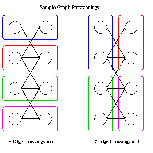
The main source of parallelism in discrete event simulation arises from partitioning the system into its physical components and having separate processors simulate each component. In the case of digital circuits, one can assign connected subcircuits to separate subprocessors. If one subcircuit is connected to another subcircuit, the corresponding processors must communicate with one another. There are many ways one could imagine assigning subcircuits to processors (two are shown in the figure below) and we need to consider how to choose a good one. In the case of elevator simulations, one can imagine a separate processor for each elevator, or one processor for each floor. Again, we need a criterion for choosing a particular partitioning and assignment.

Here is a simple model of a discrete event system we can use to describe partitioning. We model the system as a graph G=(N,E), with nodes N and edges E connecting them. Each node represents a physical component (like a subcircuit) to be assigned to a processor, and each edge represents a direct dependence between components (like a wire). Furthermore, each node n has a weight W_n representing the work required to simulate it, and each edge e has a weight W_e representing how much information must be passed along it. A natural set of goals for partitioning nodes to processors are the following.
For example, in the above figure ovals are drawn around nodes to be assigned to the same processor. Each partitioning shown assigns two nodes each to four processors. The partition on the left only has 6 edges crossing processor boundaries, whereas the partition on the right crosses ten, so assuming each edge has the same weight, the left partitioning requires less communication and so is superior.
This graph partitioning problem is a central one in graph theory and parallel computing. It is NP-complete, and so we can only expect approximate solutions in general. Rather than provide solutions now, we will continue our tour of parallelism in simulation, and treat this problem in detail in a later lecture.
Synchronous and asynchronous simulations differ in the way one schedules the updates of each subsystem, i.e. the order in which the processors may update the part of the system they own. When doing synchronous simulation, scheduling is easy: all processors update their subsystems by one time step, and then exchange information with other processors. This is expressed in the following simple loop:
   repeat
      compute locally to update local subsystem
      barrier()
      exchange state information with neighbors
   until done simulating
(Instead of a barrier, which forces all processors to wait for the slowest one, one could imagine having each processor wait just for the inputs it needed, as well as send its outputs to the processors it knows will need them. But if one processor gets sufficiently far ahead of, or behind, the other processors, this will cause messages to backup somewhere in the system (a flow control problem), so some more sophisticated synchronization will in fact be needed.)
Scheduling asynchronous simulation is yet more complicated, because different processors may be updated to different times, depending on which events have occurred. The simplest kind of asynchronous simulation is conservative, where a processor may only simulate up to time t if all relevant events up to time t from all other processors have arrived. As an example, consider simulating combinatorial logic, where the events propagate in one direction through the circuit, without any feedback. In this case, any circuit component, such as an "or gate", can change its output as soon its inputs have changed, because we know the inputs can only change once. The event graph data structure in Multipol, discussed in the last lecture, supports this kind of parallelism (once partitioning has been done). To see how to use the event graph to parallelize digital circuit simulation, see "Portable Runtime Support for Asynchronous Simulation", by Chih-Po Wen and Katherine Yelick.
As an alternative to waiting for all other events up to time t to arrive before proceeding to time t, a processor could boldly assume no such event will arrive, and simulate ahead anyway. Since this assumption might be wrong, old state information must be saved to permit backing up to a correct state. This offers a second source of parallelism, called speculative parallelism, which should be used if the conservative approach yields too little parallelism.
A simple example of this kind of parallelism, with which most graduate students eventually become familiar, is scheduling a qualifying exam. For lack of distributed calendar software, each graduate student is expected to contact 4 faculty members asynchronously, and find a common meeting time. The student will typically agree on a time with a few faculty members, and later discover that the last faculty member can't make it, requiring the other faculty members to readjust their calendars. This may happen repeatedly. Another example occurs when the central administration tries to schedule classrooms based on assumptions about class sizes.
A more interesting example of speculative parallelism occurs in some superscalar computer architectures, in an attempt to execute code more quickly. Superscalar architectures attempt automatically to execute instructions simultaneously if there are no dependencies between them, such as one instruction using a register computed by a previous instruction. We saw this on the IBM RS6000/590, which could execute up to 6 instructions at the same time. If a conditional branch occurs in a program, then often one cannot execute past this point, since one can't always predict which way it will go. Some new architectures will try to guess which way the branch will go, based on statistics from past performance, and execute ahead speculatively anyway, saving enough state to back up if necessary. For example, at the end of a loop, it is good guess that the branch will be back to the top of the loop. Other architectures may even execute both possible instruction streams that could follow the branch, and later throw one away.
Backing up is expensive for three reasons: it wastes the time used to compute an erroneous sequence of system states, it wastes the space necessary to save enough old state information to permit backing up (not so important for scheduling quals, but much more so in other situations), and it may result in idle time for processors waiting for another processor to backup and recompute. Speculation is an effective parallelization scheme only if one seldom has to backup and restore.
Multipol contains a distributed data structure called a speculative object layer which supports this kind of simulation. Given a partitioning, it handles all messages, including those which announce the need to back up. The user need only supply a simulation routine for each component, a routine to save or checkpoint the state, and a routine to restore an old state if necessary. To see how to parallelize digital circuit simulation using the speculative object layer, see the following paper by Wen and Yelick.
The force that moves each particle can typically be broken into 3 components:
force = external_force + nearby_force + far_field_force
The external force in Sharks and Fish is the current. It can be evaluated independently for each particle without knowledge of the other particles, and so in an embarrassingly parallel fashion. Effective parallelization requires that each processor own an approximately equal number of particles.
The nearby_force refers to forces depending only on other particles very close by. In the bouncing ball assignment, the force of collisions falls in this category. On a freeway, the behavior of a car depends (one hopes) on the behavior of nearby drivers, especially the one immediately ahead. In a molecule, the strongest forces on an atom may be from the other atoms to which it has a direct chemical bond. Effective parallelization requires locality, i.e. that it be likely that the nearest neighbors of a particle reside on the same processor as the particle.
A far field force depends on every other particle in the system, no matter how distant. These forces are generically of the form
far_field_force on particle i = sum_{j=1 to n except i} force(i,j)
where force(i,j) is the force on particle i due to particle j.
Gravity is an example, which appears in Shark and Fish 2, 5 and 6.
Electrostatic force is another example. The interactions of vortices in
fluid flow is another. At first glance, these kinds of forces appear to
require global communication at every step, defeating any attempt to
maintain locality and minimize communication. But there are a number of
clever algorithms to overcome this.
Sometimes a force could potentially be classified as nearby or far field. For example, the van der Waals force between atoms is a weak attraction when atoms are at least a few atomic diameters apart. It decreases like 1/r^6, where r is the distance between atoms. This function decreases so rapidly as r grows, that it can simply be ignored when r is large enough, making it a nearby_force and so less work to compute. Gravitational and electrostatic forces obey an inverse-square law, and so decrease as 1/r^2 as r grows. The function 1/r^2 decreases much more slowly than 1/r^6, and cannot be ignored for any r, if it is the only force being simulated.
There are two obvious ways to try to partition the particles among processors to compute the external_force and the nearby_force. The best way to partition for parallelizing the external force computation is to partition by particle number, or simply assigning an equal number of particles to each processor by particle number, independent of how their physical locations may change. This is how we parallelized Sharks and Fish problems 1 and 2. This guarantees perfect load balance, but is inappropriate for nearby_forces, because no locality is guaranteed. A better way to partition for nearby-forces is to partition the physical space in which the particles reside, which each processor being responsible for the particles that happen to reside in the part of space it owns. This is how we parallelized the bouncing balls assignment.
As we saw in the bouncing balls assignment, partitioning the physical space requires communication only of particles near the boundaries of the partitions. If particles are uniformly distributed, this means there is a surface to volume effect, which tends to make the amount of communication relatively small compared to the amount of computation for large numbers of particles, yielding good efficiency. For example, suppose we partition 3D space into unit cubes, that a particular unit cube contains n uniformly distributed particles, and that only the particles within distance r << 1 of the surface of the cube need to be communicated to neighboring processors. Then one expects to communicate c = 6*r*n particles, but do local work on n>>c local particles. In other words, the local computation is done with all the particles in the volume of the cube, but communication only with the much smaller of particles near the surface.
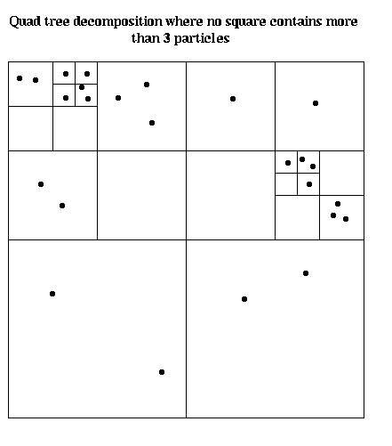
Unfortunately, if particles are not uniformly distributed, and we use a fixed partitioning of physical space, say into equal sized squares or cubes, the particles may move so as to collect in a small number of processors, ruining the load balance. This is often the case in computational fluid dynamics (CFD) using the vortex method, where turbulence and other fluid motions causes the vortices (particles) to cluster. It also arises in astrophysics, where stars tend to clump into galaxies and other large space structures, rather than be uniform (indeed, this is precisely the behavior astrophysicists want to study). This leads us to dynamic partitioning schemes based on quad-trees in 2D and oct-trees in 3D. An example is shown below, where we subdivide the plane recursively into smaller boxes, until each box contains an equal number of particles. This decomposition must be updated periodically as particles change their positions.
Now we consider parallelizing the far_field force. Since these forces are so common and important, a number of clever algorithms have been devised for reducing their algorithmic complexity, not just of the parallel algorithm, but of the serial algorithm too. The obvious serial algorithm above takes O(n^2) work for n particles. If nothing special is known about the force function force(i,j), nothing more can be done. But for forces like gravity, electrostatics and others, there is a great deal of structure in the force function, permitting us to reduce the complexity from O(n^2) to O(n log n) or even O(n), depending on the accuracy of the approximation we desire. In other words, if we are willing to trade accuracy for speed, we can significantly reduce the complexity. In practice, one can straightforwardly make the error smaller than machine precision if one wishes, so the simulation can be done as accurately as with the direct method. For some simulations less accuracy than full machine precision is good enough, and one can go even faster.
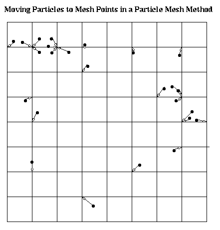
We will look at two kinds of fast methods for computing gravitational (or electrostatic) forces on n particles. We sketch them here, and return to them in detail later in the course. The first is the particle-mesh method. This method superimposes a regular grid over the set of particles, and creates an approximation of the original problem by moving particles to the nearest grid points, as shown below (more accurate interpolatory methods may be used in practice). Since this approximate problem lies on a regular grid, there are several clever divide-and-conquer solutions available for its rapid solution, such as Multigrid and the FFT. The accuracy of this approximation depends on how fine a grid we choose, and how uniformly distributed the particles are.
The second kind of method also uses divide-and-conquer, but on the original particles, without an artificial mesh. The two algorithms in this class are the Barnes-Hut algorithm and the fast multipole method; they use a similar divide-and-conquer division of space with a quad-tree (in 2D) or oct-tree (in 3D) as described above. The basic idea is that the gravitational force of a large cluster of particles, provided it is far enough away, can be approximated by a point mass at the center of mass of the particles. This lets us "compress" the information in a distant cluster of particles, and both compute with and communicate it faster. The quad-tree (or oct-tree) is used to decide which particles can be clustered and compressed in this way.
Rather than discuss these algorithms now, we will continue our tour of parallelism in simulations, and treat them in detail later.
        [ 0       A        0   ]   [ v_n ]   [ 0 ]   ... Kirchoff's Current Law
        [ A'      0       -I   ] * [ i_b ] = [ S ]   ... Kirchoff's Voltage Law
        [ 0       R       -I   ]   [ v_b ]   [ 0 ]   ... Ohm's Law
        [ 0      -I    C* d/dt ]             [ 0 ]   ... capacitance
        [ 0    L* d/dt     I   ]             [ 0 ]   ... inductance
The matrices A, R, C, L and S are sparse matrices representing the connectivity
of the circuit, and in interesting circuits they are also large matrices.
For example, A has one row for each node and one column for each branch, with
A(n,b) = +-1 if node n is one of the endpoints of
branch b, and zero otherwise (each branch is given an arbitrary orientation,
so one endpoint node is +1 and one is -1). Similarly, R has one row and
one column for each branch, with R(b,b) equaling the resistance of branch b.
C is a similar large diagonal matrix of capacitances, and L of inductances.
S is a vector of voltage sources.
This is a system of simultaneous algebraic equations (like A'*v_n = v_b) with ordinary differential equations (ODEs) (like i_b = C*dv_b/dt). The equations can be nonlinear if the resistances R, capacitances C, or inductances L depend on the values of v or i flowing through them (this is how we could model diodes, for example). A circuit simulator updates the values of v_n(t), i_b(t) and v_e(t) from time step t to time step t + dt using these governing equations.
(Our simple circuit model can only handle passive circuits, because each component -- resistors, capacitors, etc. -- has just 2 connecting wires. Active circuits, which would include transistors, require components with three wires (e.g. drain, source, and gate for transistors)).
Another example is structural analysis in civil engineering. In the simplest example the variables are the displacements of particular points or nodes in a building or other structure from their equilibrium positions. The structure may be modeled by giving these points the masses of structural members (like walls and girders), and connecting them with rigid members or perhaps stiff springs, which model the flexibility in the structural members. The governing equations are just Newton's laws and Hooke's spring law, which says that the force exerted by a spring is proportional to how much it is stretched or compressed. In static modeling, one exerts external forces on certain nodes and asks for the displacement of the other nodes; in particular one might ask whether the breaking strength of some structural member is exceeded. In dynamic modeling, one would subject certain nodes to continuous forces (from a simulated earthquake, for example), and ask how the structure moves in time. The static problem involves solving a system of algebraic equations, and the dynamic problem a system of differential equations. As in the case of circuits, the matrices are large and sparse, where the sparsity structure (which entries are nonzero and which are zero) depending on which structural members are connected to which other members.
A third example is chemical kinetics, or computing the concentrations of chemicals undergoing a reaction. To illustrate, suppose we have three chemicals O (atomic oxygen), O3 (ozone) and O2 (normal molecular oxygen). A very simple model (which we borrow from the book "Numerical Methods and Software" by Kahaner, Moler and Nash) for photochemical smog in cities like Los Angeles, consists of the 4 reactions
      (1)      O + O2 --> O3
      (2)      O + O3 --> 2O2
      (3)          O2 --> 2O
      (4)          O3 --> 0 + O2
In addition, each reaction i has a rate constant ki, which says how
"fast" the reaction occurs. Given this information, it is straightforward to
produce a system of ODEs for the concentration of each chemical.
We let [O], [O2] and [O3] denote the concentrations (in moles per liter,
atoms per cubic inch, or some similar units) that we wish to compute as
functions of time. We suppose the reactions occur in a "well stirred
container", so all chemicals are uniformly distributed. In this case,
one can interpret the concentration [O] of O as the probability
of finding an atom of O in a fixed tiny volume. For O and O2 to
react, both must simultaneously be in the same tiny volume.
Since O and O2 are well-stirred, i.e. independently distributed, the chance
that a single atom or molecule of each is simultaneously present is the
product of the probabilities, [O]*[O2]. Given that both are present,
the reaction rate k1 measures the chance that the reaction actually occurs.
If it occurs, one molecule of O3 is created, and one each of O and O2 is
destroyed. This leads to the following ODEs, which model just the first reaction
above:
      d [O3]/dt = +k1*[O]*[O2]
      d [O]/dt  = -k1*[O]*[O2]
      d [O2]/dt = -k1*[O]*[O2]
To incorporate the second reaction into the ODEs, we reason similarly.
Thus we get an additional term of
-k2*[O]*[O3] for the equations for d [O3]/dt and d[O]/dt, since
one atom/molecule each of O and O3 are consumed, and a
+2*k2*[O]*[O3] term for the equation for d[O2]/dt, since two molecules
of O2 are created. This yields the following ODEs for the first 2 reactions:
      d [O3]/dt = +k1*[O]*[O2] - k2*[O]*[O3]
      d [O]/dt  = -k1*[O]*[O2] - k2*[O]*[O3]
      d [O2]/dt = -k1*[O]*[O2] + 2*k2*[O]*[O3]
Treating reactions 3 and 4 similarly yields the complete set of ODEs
for all four reactions:
      d [O3]/dt = +k1*[O]*[O2] - k2*[O]*[O3] - k4*[O3]
      d [O]/dt  = -k1*[O]*[O2] - k2*[O]*[O3] + 2*k3*[O2] + k4*[O3]
      d [O2]/dt = -k1*[O]*[O2] + 2*k2*[O]*[O3] - k3*[O2] + k4*[O3]
The most complete model of smog in Los Angeles includes 92 chemical
species participating in 218 reactions (Mark Jacobsen, PhD Thesis,
Dept. of Atmospheric Sciences, UCLA, 1994). This is represented
as a sparse matrix with one row and one column for each chemical,
and a nonzero entry at (i,j) if chemicals i and j react.
Now we discuss the sources of parallelism in these problems. Even though we have differential equations and nonlinear systems to solve, the computational bottlenecks all reduce to linear algebra with sparse matrices. The simplest example is solving a system of linear algebraic equations A*x=b. There are a variety of methods available for this, including sparse Gaussian elimination among many others we will later discuss. The second example is solving a nonlinear system of equations, which we write as f(x)=0. The most common method for its solution is Newton's method, which we write as
x(i+1) = x(i) - inv(df(x(i))/dx)) * f(x(i))
Here df(x(i))/dx is the Jacobian matrix of first partial derivatives
of f evaluated at x(i).
If x(i) is an n-dimensional vector, then df/dx is an n-by-n matrix,
and taking one step of Newton's method requires the solution of the
linear system of equations
df(x(i))/dx * (x(i+1)-x(i)) = f(x(i))
Now we turn to the solution of ODEs. For simplicity, we consider the simple model problem dx/dt = A*x(t), where A is a matrix which could depend on time. In order to understand the computational bottlenecks, we look at the two simplest solution methods: Euler's Method and Backward Euler's Method. More sophisticated methods are often used, but these are good enough to illustrate the computational bottlenecks. In both cases, we use a fixed time step h, in other words we only attempt to approximate the solution at t=0, h, 2*h, ... , i*h. More sophisticated methods would use a variable time step, taking big steps where the solution is smooth and so easy to compute, and small steps where it is changes rapidly and so is hard to compute.
Euler's method approximates the derivative dx(t)/dt by the divided difference
                 x( t+h ) - x( t )
      dx(t)/dt ~ -----------------
                         h
If we take the limit as h goes to zero, the right-hand-side approaches the
derivative dx(t)/dt, so this is a reasonable approximation to make if h
is small enough. Now substitute this approximation for dx(t)/dt in the ODE to get
     x( t+h ) - x( t )
     ----------------- = A*x( t )
             h
Assuming we know the approximate solution for x( t ), we can solve for
x( t+h ) to get
x( t+h ) = x( t ) + h*A*x( t )
This is Euler's method, and provides a simple formula for computing the
approximate solution at time t+h, given the solution at time t. Using
this we can step forward in time as long as we like. The computational
bottleneck is the sparse matrix-vector multiplication A*x.
Sometimes Euler's method requires a very small time step h in order to get reasonable accuracy, even when the solution is smooth. This happens, for example, if the ODE has a property called stiffness, which means the solution vector x(t) has some components which change rapidly and others which change smoothly, and we are only interested in the smoothly changing components. Stiff ODEs occur commonly in chemical kinetics and some circuit simulations. For these problems, the method of choice is Backward Euler:
     x( t+h ) - x( t )
     ----------------- = A*x( t+h )
             h
Note that we have changed the right-hand-side from A*x(t) to A*x(t+h). Solving for x( t+h )
yields
(I - h*A) * x( t+h ) = x( t )
a linear system of equations to solve for x( t+h ). This is the computational
bottleneck.
Thus sparse matrix-vector multiplication and solving a sparse system of linear equations are the computational bottlenecks we need to parallelize. Here we content ourselves with showing that a good parallel algorithm for sparse matrix-vector multiplication depends on solving the graph partitioning problem discussed earlier.
Let the problem to parallelized be multiplying y=A*x, where A is n-by-n and sparse. We need to decide
Suppose we partition N as the union of N1 through Np, where p is the number of processors. Assigning Ni = to processor i will mean that
This is an example of the owner computes rule, where we let the processor owning y(k) perform all the computations required to compute it (one could imagine other possibilities as well).For example, the following figure illustrate a particular 8-by-8 sparse matrix and a particular partitioning onto 4 processors.
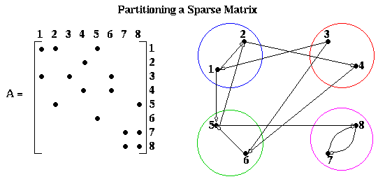
Using this machinery, we can state the graph partitioning problem as choosing a partition of N into the union of N1 through Np such that
A last linear algebra problem that arises in solving ODEs is the following. Suppose that in dx(t)/dt = A*x(t), matrix A is constant, independent of x or t. In this simple but important case, we can "guess" a solution x(t) = exp(z*t)*x0, where z is a constant scalar to be determined, and x0 is a nonzero constant vector to be determined. Plugging into the ODE yields
dx(t)/dt = z * exp(z*t) * x0 = A * exp(z*t) * x0
Canceling exp(z*t), which is always nonzero, yields
z * x0 = A * x0
which is an eigenvalue problem we can solve for z and x0.
Later we will discuss solution techniques for eigenproblems.
All the methods for ODEs discussed above advance the solution x(t) from time step t to time step t+h. In other words, there is no parallelism in time, which would let us compute the solution at a distant future time T without computing the solution at all the intermediate times, in a sequential fashion. (In the very special case of a linear ODE, dx/dt = A(t)*x(t) + b(t), it is actually possible to use parallel prefix to solve it in time O(log(T/h)) instead of O(T/h), but I have not seen this used in practice.) There is a completely different technique that does not require sequential time stepping, and so offers the possibility of parallelism in time as well as in a simple step. This technique is called waveform relaxation. It starts with a guess for the solution on the entire time interval of interest, say [0,T], and iteratively improves it, converging at every time step simultaneously. For some special ODEs, it converges rapidly enough to compete with methods like Euler and Backward Euler. But methods like Euler and Backward Euler are used much more commonly.