We think of a node n in N as representing an independent job to do, weight W_n as measuring the cost of job n, and an edge e=(i,j) in E as meaning that an amount of data W_e must be transferred from job i to job j to complete the overall task. Partitioning G, which was introduced in Lecture 16 , means dividing N into the union of P disjoint pieces
N = N1 U N2 U ... U NPwhere the nodes in Ni are assigned to be done by processor Pi. This partitioning is done subject to the optimality conditions below.
We present a variety of useful algorithms for solving this problem. For simplicity, we will present most of them with unit weights W_n = 1 and W_e = 1, although most can be generalized to general weights.
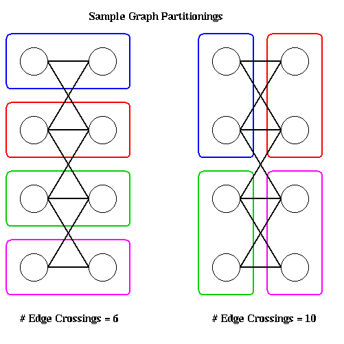
To illustrate, the following figure shows two partitions of a graph with 8 nodes onto 4 processors, with 2 nodes per processor. The partitioning on the left has 6 edges crossing processor boundaries and so is superior to the partitioning on the right, with 10 edges crossing processor boundaries. The reader is invited to find another 6-edge-crossing partition, and show that no fewer edge crossings suffice.

In general, computing the optimal partitioning is an NP-complete problem; it is equivalent to the max-cut problem, as we will later describe. Therefore we need to use heuristics to get approximate solutions.
There are two classes of heuristics, depending on the information available about the graph G. In the first case, we have coordinate information with each node, such as (x,y) or (x,y,z) coordinates. This is frequently available if the graph comes from triangulating or otherwise discretizing a physical domain. For example, in the NASA Airfoil, there are (x,y) coordinates associated with each node (to see the data and be able to manipulate it, start up matlab and type "airfoil"). Typically, such graphs have the additional property that only nodes which are spatially close together have edges connecting them. We may use this property to develop two efficient geometrical algorithms for graph partitioning.
The second kind of graph we want to partition is coordinate free, i.e. we have no identification of a node with a physical point in space. In addition, edges have no simple interpretation such a representing physical proximity. These kinds of graphs require other algorithms to be used (which may obviously also be applied to graphs with coordinate information).
Almost all the algorithms we discuss are only for graph bisection, i.e. they partition N = N1 U N2. They are intended to be applied recurively, bisecting N1 and N2, etc, until the partitions are small and numerous enough.
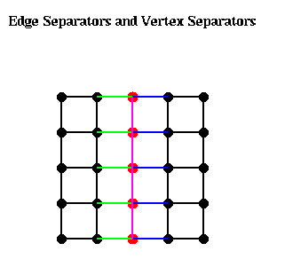
The other way to bisect a graph is to find a vertex separator, a subset Ns of N, such that removing Ns and all incident edges from G also results in two disconnected subgraphs G1 and G2 of G. In other words N = N1 U Ns U N2, where all three subsets of N are disjoint, N1 and N2 are equally large, and no edges connect N1 and N2.
The following figure illustrates these ideas. The green edges, Es1, form an edge separator, as well as the blue edges Es2. The red nodes, Ns, are a vertex separator, since removing them and the indicident edges (Es1, Es2, and the purple edges), leaves two disjoint subgraphs.
Given an edge separator Es, one can produce a vertex separator Ns by taking one end-point of each edge in Es; Ns clearly has at most as many members as Es. Given a vertex separator Ns, on can produce an edge separator Es by taking all edges incident to Ns; Es clearly has at most d times as many members as Es, where d is the maximum degree (number of incident edges) of any node. Thus, if d is small, finding good edge separators and good vertex separators are closely related problems, a fact we exploit below.
|S| = m = sqrt(m^2) = sqrt(number of nodes).It turns out that it is generally possible to find a vertex separtor containing about the square root of the number of nodes.
Theorem. (Tarjan, Lipton, "A separator theorem for planar graphs", SIAM J. Appl. Math., 36:177-189, April 1979). Let G=(N,E) be an planar graph. Then we can find a vertex separator Ns, so that N = N1 U Ns U N2 is a disjoint partition of N, |N1| <= (2/3)*|N|, |N2| <= (2/3)*|N|, and |Ns| <= sqrt(8*|N|).
In other words, there is a vertex separator Ns that separate the nodes N into two parts, N1 and N2, neither of which can be more than twice as large as the other, and Ns has more more than about the square root of the number of nodes. This intuition motivates the algorithms below.
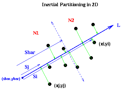
It remains to show how to pick the line L. Intuitively, if the nodes are located in a long, thin region of the plane, as in the above example, we want to pick L along the long axis this region:
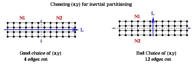
In mathematical terms, we want to pick a line such that the sum of squares of lengths of the green lines in the figure are minimized; this is also called doing a total least squares fit of a line to the nodes. In physical terms, if we think of the nodes as unit masses, we choose (x,y) to be the axis about which the moment of inertia of the nodes is minimized. This is why the method is called inertial partitioning. This means choosing a, b, xbar and ybar so that a^2 + b^2 = 1, and the following quantity is minimized:
     sum_{i=1}^{|N|} (length of i-th green line)^2
   = sum_{i=1}^{|N|} ((xi-xbar)^2 + (yi-ybar)^2 - (-b*(xi-xbar) + a*(yi-ybar))^2 )
        ... by the Pythagorean theorem
   =   a^2 *   ( sum_{i=1}^{|N|} (xi-xbar)^2 )
     + b^2 *   ( sum_{i=1}^{|N|} (yi-ybar)^2 )
     + 2*a*b * ( sum_{i=1}^{|N|} (xi-xbar)*(yi-ybar) )
   = a^2 * X2 + b^2 * Y2 + 2*a*b * XY
   = [ a b ] * [ X2  XY ] * [ a ]
               [ XY  Y2 ]   [ b ]
   = [ a b ] * M * [ a ]
                   [ b ]
where X2, Y2 and XY are the summations in the previous lines.
On can show that an answer is to choose
   xbar = sum_{i=1}^{|N|} xi / |N|
   ybar = sum_{i=1}^{|N|} yi / |N|
i.e. (xbar,ybar) is the "center of mass" of the nodes,
and (a,b) is the unit eigevector corresponding to the smallest eigenvalue of the matrix M.
The 3D (and higher) case is similar, except that we get a 3-by-3 matrix whose eigenvector we need.
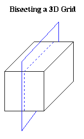
To extend our intuition about planar graphs to higher dimensions, we need a notion of graphs that are well-shaped in some sense, so that the cells created by edges joining nodes (triangles in 2D, simplices in 3D, etc.) cannot have angles that are too large or too small. The following approach is taken by G. Miller, S.-H. Teng, W. Thurston and S. Vavasis ("Automatic mesh partitioning", in Graph Theory and Sparse Matrix Computation, Springer-Verlag 1993, editted by J. George, J. Gilbert and J. Liu). Our presentation is drawn from "Geoemtric Mesh Paritioning" by J. Gilbert, G. Miller and S.-H. Teng (available from gilbert@parc.xerox.com).
Definition. A k-ply neighborhood system in d dimensions is a set {D1,...,Dn} of closed disks in d-dimensional real space R^d, such that no point in R^d is strictly interior to more than k disks.
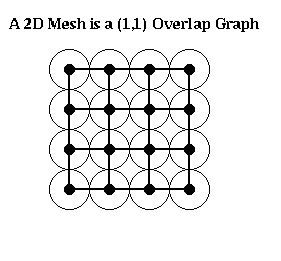
Definition. An (alpha,k) overlap graph is a graph defined in terms of a constant alpha >= 1, and a k-ply neighborhood system {D1,...,Dn}. There is a node for each disk Di. There is an edge (i,j) if expanding the radius of the smaller of Di and Dj by a factor alpha causes the two disks to overlap. For example, an n-by-n mesh is a (1,1) overlap graph, as shown below. The same is true for any d-dimensional grid. One can show any planar graph is an (alpha,k) overlap graph.
One can prove the following generalization of the Lipton-Tarjan theorem:
Theorem. (Miller, Teng, Thurston, Vavasis). Let G=(N,E) be an (alpha,k) overlap graph in d dimensions with n nodes. Then there is a vertex separator Ns, so that N = N1 U Ns U N2, and
The separator is constructed by choosing a sphere in d-dimensional space, using the edges it cuts as an edge separator, and extracting the corresponding vertex separator. There is a randomized algorithm for choosing the sphere from a particular probability distribution such that it satisfies the conditions of the theorem with high probability.
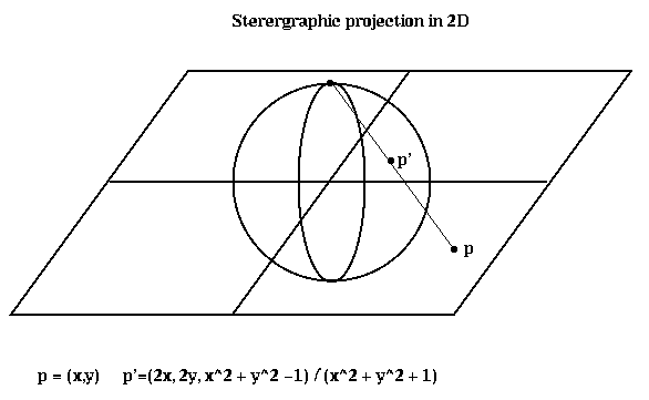
To describe the algorithm, we need to explain stereographic projection, which is a way of mapping points in a d-dimensional space to the unit sphere centered at the origin in (d+1) dimensional space. When d=2, this is done by drawing a line from the point p to the north pole of the sphere; the point p' where the line and sphere intersect is the stereographic projection of p. The same idea applies to higher dimensions.
Here is the algorithm. Matlab software implementing it is available via anonymous ftp from ftp.parc.xerox.com at /pub/gilbert/meshpart.uu.