Discussion Section 3
Scan Conversion Distillation

Overview

These are the issues discussed in this discussion section:

Introduction (who am I)
Review of definitions
Polygon fill rules
Two approaches to Scan Conversion
1. Triangulate, render trangles
2. General Purpose (e.g. Sample-Point algorithm)
Assignment 3 - Interactive Viewer for 3-D Convex Objects

0. Introduction (who am I)

I am a 29-year-old 7th-year Computer Science graduate student at the University of California at Berkeley. I work with Prof. Brian A. Barsky in the OPTICAL project, and I'm in charge of the Scientific Visualization component of the research. When I graduate, I hope to acquire an academic position in a teaching college in the Northeast US (hopefully NY!). This is the seventh time I've taught cs184 (Fa92, Sp93, Fa93, Fa94, Sp96, Fa96, Fa97).

1. Review of definitions

Here we review terms and definitions from the scan conversion lecture.

1.1 What is scan conversion, really?

Scan conversion is the method we use to specify which pixels to fill and what to fill them with. We have primitives stored internally (polygons, lines, characters, etc.) and we would like to be able to render them on the screen. We need to convert them to pixels which we learned about in the previous lecture. Figure 1 shows a simple overview of this:

Figure 1 - The Overview of Scan Conversion

This discussion section is intended to distill some confusion that inevitably results when learning this topic for the first time. Let's first focus on some of the terminology that you've heard thrown around and make sure these are clear.

1.2 What is a scan line?

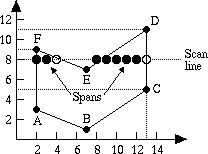
A scan line is a line of constant y value which we use to generate spans.

1.3 What is a span?

A span is the collection of adjacent pixels on a single scan line which lie inside the primitive. Said another way, they are the pixels which reside between a pair of edges and are inside the polygon, in our case. We linearly interpolate attributes such as depth or color between the values at the two edges to get a nice, smooth result within the polygon.

1.4 What is spatial coherence?

Coherence literally means to be logically consistent or connected, and in this context means that primitives don't change an awful lot if at all from pixel to pixel within a scan line or from scan line to scan line. This allows us to optimize our algorithms.

1.5 What is edge coherence?

Edge coherence means that most of the edges that intersect scan line i also intersect scan line i+1. Since our polygons are defined by straight lines, we can incrementally calculate the new x intersection from the previous one. We will see this for many attributes, specifically color, z-value and x-value (where an edge intersects a scan-line).

1.6 What is a convex polygon?

Convex polygons have the property that intersecting lines cross it either one (crossing a corner), two (crossing an edge, going through the polygon and going out the other edge), or an infinine number of times (if the interesecting line lies on an edge). Figure 2 shows these cases for a single convex polygon. If that intersecting line happens to be a scan line, that means that there is no more than one span of pixels. Triangles are the only polygons which are guaranteed to be convex and planar, and we'll say why this is important later in the course.

Figure 2 - A convex polygon and an intersecting scan line crossing it once, twice and an infinite number of times

1.7 What is a concave polygon?

Concave polygons don't have the nice properties of convex polygons, and are thus more complicated. An intersecting line may cross it any number of times. Unless we tell you that an algorithm requires its input polygons to be convex, assume the input can be concave polygons. If you ever have trouble remembering which is which, think of the phrase: "caving-in".

Figure 3 - A convex polygon and a scan line crossing it four times

2. Polygon fill rules

The basic scan-line algorithm is to traverse the scan lines from top to bottom and find the intersections of the scan line with all edges of the polygon. The data structure that keeps an ordered list (sorted by the intersection with the current scanline) of all active edges on any particular scan line is called the Active Edge List (AEL) (also called the Active Edge Table (AET)). Then, using this list, determine if a particular pixel is either inside the polygon or outside based on certain criteria. Let us look at three criteria for pixel inclusion within one scan line: the odd-even (or parity) rule, the nonzero winding rule, and the nonexterior rule.

2.1 Odd-even (or parity) rule

Begin from a point which is outside the polygon and define (and initialize) a variable which we'll call number_of_edges_crossed_so_far to be zero. Increase the x value and add one to number_of_edges_crossed_so_far for every edge we cross on that scan line. Then use the following criteria for pixel inclusion or exclusion:

A pixel is inside the polygon if number_of_edges_crossed_so_far is odd, and outside if number_of_edges_crossed_so_far is even. This method is known as the odd-even rule, and it also works for self-intersecting polygons as we see in figure 5. Seems to work for scan line number 8 in figure 4, and for the polygon in figure 5, doesn't it?

Figure 4 - A polygon and scan line 8 (from figure 3.14 of page 87 of Computer Graphics Principles and Practice by Foley, VanDam, Feiner & Hughes)

Figure 5 - The Odd-even (or parity) rule

2.2 Nonzero winding rule

The winding rule is not difficult, conceptually or in practice. The idea is to determine if a given pixel in the image is inside or outside. The answer is that it's outside if we calculate zero windings, and inside otherwise. Now all we need it to figure out how to calculate windings. It's simple.

An easy mnemonic is that zero ends with an 'o', and outside begins with an 'o', so we can write zeroutside.

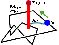
Think of the polygon as a path in the snow that someone has left. There is a flagpole sitting on a point in the region in question, and a rubber band connecting you to the flagpole. You traverse the snow path completely and finish back at where you started. If when you look at the flagpole the rubber band has been wrapped around once, then you have a winding of one. The winding number is negative if it's wrapped clockwise. If its final position is the same as its initial position, then you have zero windings and it's outside the polygon! (remember zeroutside) Try this out for several points in different regions in figure 5 to convince yourself. Figure 6 illustrates the walk-in-the-snow-around-a-flagpole method for calculating the winding number.

Figure 6 - The walk-in-the-snow-around-a-flagpole method of calculating the winding number

An easier way of thinking about the winding rule conceptually is to think of putting your finger in the point in question. If it's possible to pull the polygon away (imagine that the polygon's edges are traced in string on a table) then the point is outside, otherwise it's inside. This is a much faster method than the previous. Try this for several self-intersecting polygons to convince yourself.

How does one implement a guy walking in the snow with a rubber band tied to his behind in C? Aha! We're glad you asked. (This is paraphrased from page 965 in Computer Graphics: Principles and Practice if you are confused by my explanation). First, we must note that it's important to order the directions of the edges so that you could walk around the snowy path (in either direction) always going in the direction of the arrows. I.e. every edge's ending vertex is another edge's starting vertex.

Instead of keeping track of number_of_edges_crossed_so_far, as in the even/odd method, keep track of the number of edges which point upwards and downwards. Figure 7 shows examples of edges which fulfill each criteria.

Figure 7 - Upward- and downward-pointing edges

Every upward pointing edge gets a value of 1 and every downward pointing edge gets a value of -1. The sum of these numbers for every edge in the AEL is the winding number. If the sum is zero, as we recall from a couple lines before, then the point is outside, otherwise it's not. How do we determine if an edge is pointing upward or downward (think about the difference between y value of the starting and ending vertices)? Again, convince yourself of this using several small examples. Does it represent the same filling pattern as the odd-even rule did? Compare figure 8 below to figure 5 above.

Figure 8 - The Nonzero winding rule

It's important to note that the line in figure 7 doesn't have to be a scan line. It can be any curve which starts from infinitely far away and outside the polygon. Upward-pointing edges are edges that begin from the left of the curve, cross the curve (Why did the edge cross the curve? To get to the other side!), and end on the left of the curve. Similarly for downward-pointing edges.

2.3 Nonexterior rule

The nonexterior rule considers all regions in if they must cross an edge to reach a point infinitely far away. Said another way, think of the edges of the polygon as a fence to hold in animals. Any region which would successfully hold animals is considered inside the polygon. See figure 9 below for an example of the nonexterior rule. You may want to think about why you can't implement the nonexterior rule with a one-pass scan converter wtihout very intelligent pre-processing.

Figure 9 - The Nonexterior rule

WWW Maven: Dan Garcia (ddgarcia@cs.berkeley.edu)

Send me feedback

Discussion Section 3 Scan Conversion Distillation