CS 184: COMPUTER GRAPHICS
PREVIOUS
< - - - - > CS
184 HOME < - - - - > CURRENT
< - - - - > NEXT
Lecture #26 -- Wed 4/27/2011.
Warm-up for Anti-Aliasing:
|

|
A wheel with 8 spokes is turning at
a rate of 1 revolution per second.
What does the wheel appear to do
when it is rendered at 10 frames/sec.
without any anti-aliasing measures ?
|
How many B&W line pairs can you draw
on a display with 1200x1200 square pixels:
(a) vertical lines in the horizontal direction ?
(b) diagonal lines between opposite corners ?
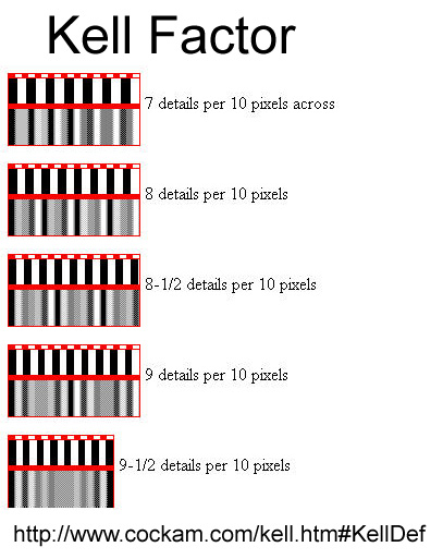
Pixel Patterns Kell Factor
|
Transparency (cont.)
Transparency measures what fraction of light passes through
a surface or body;
that fraction is indicated by the transmission coefficient kt.
Opacity (a) indicates what fraction
is held back; a=1 means: completely opaque.
By definition: kt + a = 1
Translucency is a partly transparent object in which the scattering effect dominates; example: frosted glass.
There are many ways to implement partially transparent/opaque objects:
Ray Tracing
Any of the Photon-, Path-, Beam-tracing methods discussed
are a natural way to deal with a (partially) transparent object T;
for instance:
At the surface of object T, we split the ray into a primary ray that
returns the color of object T with some weighted percentage,
and into a secondary ray that passes through the medium and returns
information "from behind" with the complementary percentage.
This information could be further attenuated or discolored, depending
on the thickness of the body T.
Alpha Channel
OpenGl offers another mechanism: alpha blending.
A fourth channel a is established
-- in addition to R, G, B.
Thus for each surface, vertex, or pixel we can define four values:
(RGBa).
If a-blending is enabled, the fourth parameter a
determines
how the the RGB values are written into the frame buffer:
typically the result is a linear combination (or blend) of the
contents already in memory and the new information being added.
Filtered Transparency:
Assume that in the frame buffer there is a pixel (Fr, Fg, Fb, Fa),
and we want to place a new pixel with opacity a
in front of it (Nr, Ng, Nb, Na):
We can achieve the desired result with: ( a*Nr
+ kt*Fr, a*Ng
+ kt*Fg, a*Nb
+ kt*Fb, a*Na
+ kt*Fa );
this corrsponds to placing a filter of opacity a
in front of an already rendered scene.
(if a=1 the New pixel dominates).
For this blending function to work, the transparent polygons have to
be rendered after (in front of) the opaque objects.
For multiple filter polygons, the effect is calculated recursively
back-to-front.
Interpolated Transparency:
In a different situation, we might want to form a composite image from m
candidate images
(e.g. m different surfaces sharing parts of one pixel; or in Image-based Rendering: interpolating between m different views).
In this case, the compositing function might look like: ( sum(Nri)/m,
sum(Ngi)/m, sum(Nbi)/m,
sum(Nai)/m, )
OpenGL provides many different blending functions to take care of many
commonly occuring situations.
Rendering with Participating Media
The intensity and color of light rays may not only be changed when they
interact with discrete surfaces.
When light
rays pass through media that are not completely transparent (water,
vapor, fog, smoke, colored glass ...),
the interaction with these media happens along the whole path,
and the resulting effect increases exponentially with the length of
the path.
(If the effect is small enough, a linear approximation can be used.)
When scenes contain smoke or dust, it may be necessary to take into account
also the scattering
of light as it passes through the media (equivalent to distributed light sources).
This involves solving the radiative transport equation (an integro-differential
equation),
which is more complicated than the traditional rendering equation solved
by global illumination algorithms.
These effects are important when rendering natural phenomena such as: Fire, Smoke, Clouds, Water ...
The photon map method is quite good at simulating light
scattering in participating media.
So far we have assumed a uniform participating medium.
Volume Rendering
Alternatively, we might want to see details throughout the whole volume.
Then we need to render all the 3D raster data like some partly transparent fog with variable opacity,
or like nested bodies of "jello" of different colors and transparencies, which can then be rendered with raytracing methods.
The Volume Rendering technique can directly display sampled 3D data without
first fitting geometric primitives to the samples.
In one approach, surface shading calculations are performed at every
voxel using local gradients to determine surface normals.
In a separate step, surface classification operators are applied to
obtain a partial opacity for every voxel,
so that contour surfaces of constant densities or region boundary surfaces
can be extracted.
The resulting colors and opacities are composited from back to front
along the viewing rays to form an image (as above).
With today's GPU's this sort of data can be
displayed in real time with almost
photorealistic quality for volume renderings
of medium-sized scientific,
engineering, or medical datasets.
Example: Scull
and Brain
Source: http://graphics.stanford.edu/projects/volume/
Sampling, Anti-Aliasing; Handling Texture Maps and Images
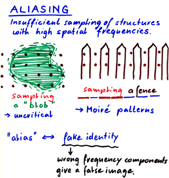
Moiré Effects
==> Demonstrate Moiré patterns with grids on VG projector.
What is going on here ? Low (spatial) frequency patterns result
from an interaction of two mis-registered grids.
What does this have to do with computer graphics ? ==> Occurs
in rendering.
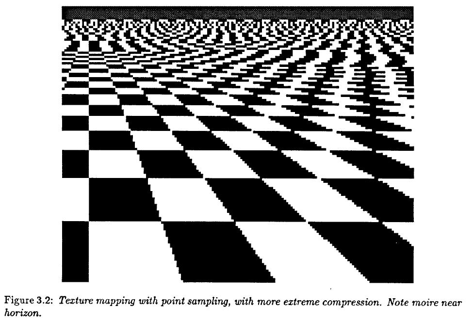
When sampling a fuzzy blob (low spatial frequencies) there is no problem, but
sampling a fence (periodic structure) at a sampling rate similar to
the lattice period will cause Moiré patterns.
Why is it called aliasing
? ==> Strong connection to signal processing!
But here we deal with a spatial/frequency domain (rather than the time/frequency domain).
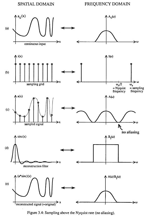
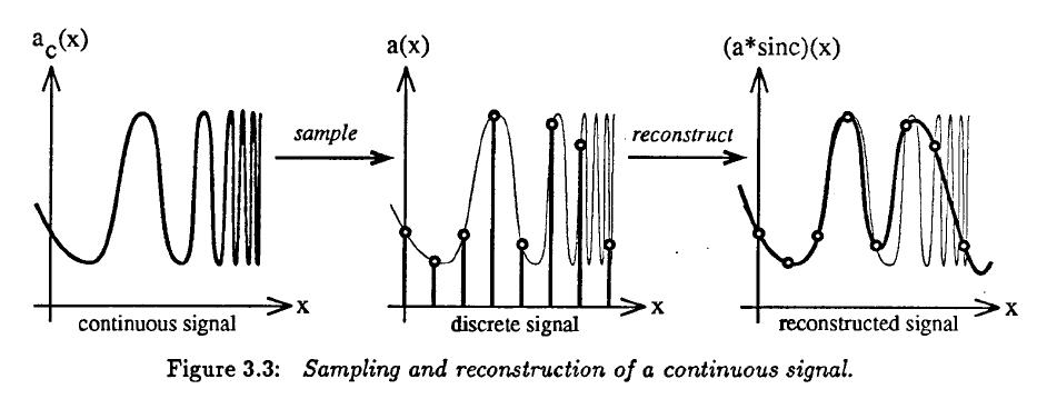
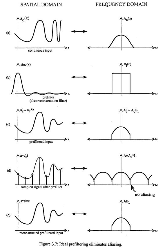
To properly resolve a high-frequency signal (or spatial structure) in a sampled environment,
we must take at least TWO samples for the highest-frequency periods of the signal. This is called the Nyquist frequency limit.
Problems arise, if our signal frequency exceeds this Nyquist limit.
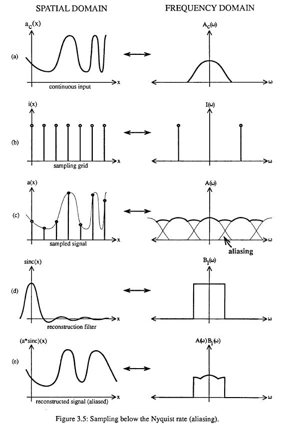
If our sampling frequency is too low, the corresponding humps in the frequency domain move closer together and start to overlap!
Now frequencies in the different humps start to mix and can no longer be separated (even with the most perfect filter!).
Thus some high frequency components get mis-interpreted as much lower frequencies;
-- they take on a different "personality" or become an a alias.
{The figures used here are from P. Heckbert's MS Thesis:
http://www-2.cs.cmu.edu/~ph/texfund/texfund.pdf }
What does a computer graphics person have to know ?
This occurs with all sampling techniques!
Rendering techniques that are particularly affected:
-- Ray-casting, ray-tracing: -- Because we are sampling
the scene on a pixel basis.
-- Texture-mapping: -- Because we use a discretely
sampled texture map.
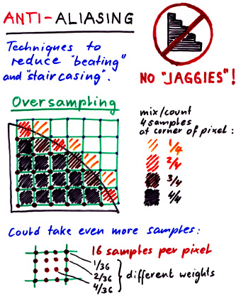
==> Fight it ! -- "NO
JAGGIES!"
-- Techniques to overcome it are
called anti-aliasing.
If we cannot increase sampling density,
then we must lower the spatial frequencies by lowpass filtering the
input -- BEFORE we sample the scene!
This cuts off the high frequency components that could cause trouble by overlapping with lower "good" frequencies.
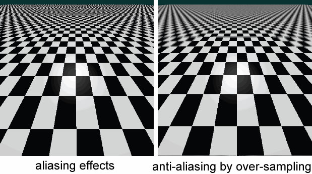
But in computer graphics we can very often get rid of aliasing by oversampling and by combining samples.
The generalization of this (multiple samples combined with different weights) is called "digital filtering."
In the context of ray-tracing we shoot multiple rays per pixel ==> Leads to "Distribution Ray Tracing".
This not only lets us gracefully filter out the higher, bothersome spatial frequencies,
it also allows us to overcome temporal aliasing problems caused by fast moving objects (e.g.. spoked wheel in warm-up question).
By taking several snapshots at different times in between subsequent frames and combining them,
we can produce "motion blur" and generate the appearance of a fast smooth motion.
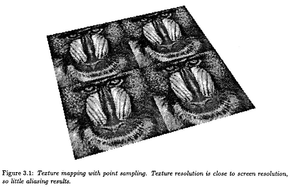
If the
frequency content of the texture pattern is close to screen resolution,
then there are no higher spatial frequencies present than what the pixel sampling can handle.
But if the texture is of much higher resolution, then there is a serious problem!
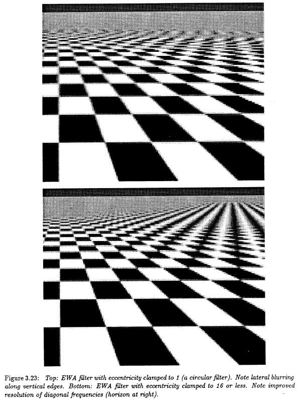
Fortunately there are filtering techniques that can fix that problem -- simple oversampling will do.
There are more advanced techniques using elliptical filtering that can give even better results.
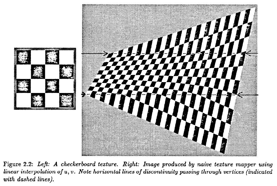
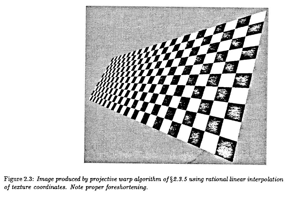
There is another issue with sampled texture patterns:
In a perspective projection, it is not good enough to determine the
texture coordinates
of the many pixels of a texture-mapped polygon simply by linear interpolation, since the
perspective projection to 2D is a non-linear operation.
If we simply linearly interpolate the texture coordinates along the edges of our polygons
(or the triangles or trapezoids that they may be cut up into), the
texture pattern will appear warped.
We need to properly foreshorten the texture coordinates with the perspective transform, so that the result will appear realistic.
In all image-based/enhanced models, sampling issues are of crucial importance.
=== END OF OFFICAL COURSE MATERIAL ===
Course Projects: Consult Project Page!
Progress Report
Oral Presentation
=== TOPICS TO BE ADDRESSED IN VARIOUS GRADUATE COURSES ===
Image-Based Rendering
Here, no 3D model of a scene to be rendered exists, only a set of images taken from several different locations.
For two "stereo pictures" taken from two camera locations
that are not too far apart,
correspondence is
established between key points in the two renderings (either manually, or with computer vision techniques).
By analyzing the differences of their relative positions in the two
images, one can extract 3D depth information.
Thus groups of pixels in both images can be annotated with a distance
from the camera that took them.
This basic approach can be extended to many different pictures taken from
many different camera locations.
The depth annotation establishes an implicit 3D database of the geometry
of the model object or scene.
Pixels at different depths then get shifted by different amounts.
To produce a new image from a new camera location, one selects
images taken from nearby locations
and suitably shifts or "shears" the pixel positions according to their
depth and the difference in camera locations.
The information from the various nearby images is then combined in
a weighted manner,
where closer camera positions, or the cameras that see the surface of interest under a
steeper angle, are given more weight.
With additional clever processing, information missing in one image
(e.g., because it is hidden behind a telephone pole)
can be obtained from another image taken from a different angle,
or can even be procedurally generated by extending nearby texture patterns.
Example 1: Stereo
from a single source:
A depth-annotated image of a 3D object, rendered from two different
camera positions.
Example 2: Interpolating an
image from neighboring positions:
To Learn More: UNC Image-Based Rendering
Future Graduate Courses: CS 283, CS 294-?
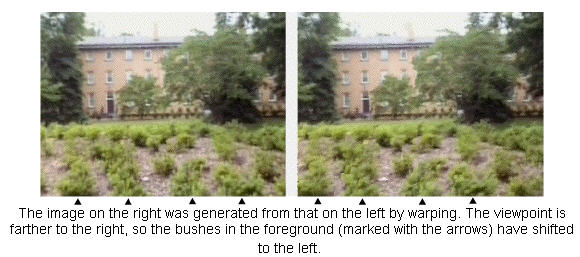
Image Warping (re-projection) and Stitching
Images taken from the same location, but at different camera angles need to be warped before they can be stitched together:
The original two photos at different angles. The final merged image.
To Learn More: P. Heckbert's 1989 MS Thesis: Fundamentals of Texture Mapping and Image Warping.
Light Field Rendering
How many images are enough to give "complete" information about all visual aspects of an object or scene ?
Let's consider the (impler) case of a relatively small, compact "museum piece" that we would like to present
to the viewers in a "3D manner" so that they can see it from (a range of) different angles.
Let's consider a few eye positions to view the crown. How many camera positions need to be evaluated ?
Light field methods use another way to store the information acquired from a
visual capture of an object.
If one knew the complete 4D plenoptic function (all the photons
traveling in all directions at all points in space surrounding an object),
i.e., the visual information that is emitted from the object in all
directions into the space surrounding it,
then one could reconstruct perfectly any arbitrary view of this object
from any view point in this space.
As an approximation, one captures many renderings from many locations
(often lying on a regular array of positions and directions),
ideally, all around the given model object, but sometimes just from
one dominant side.
This information is then captured in a 4D sampled function (2D
array of locations, with 2D sub arrays of directions).
One practical solution is to organize and index this information (about
all possible light rays in all possible directions)
by defining the rays by their intercept coordinates (s,t) and (u,v)
of two points lying on two parallel planes.
The technique is applicable to both synthetic and real worlds, i.e.
objects they may be rendered or scanned.
Creating a light field from a set of images corresponds to inserting
2D slices into the 4D light field representation.
Once a light field has been created, new views may be constructed by
extracting 2D slices in appropriate directions,
i.e., by collecting the proper rays that form the desired image, or a few close-by images that can be interpolated.
"Light Field Rendering":
Example: Image
shows (at left) how a 4D light field can be parameterized by the
intersection of lines with two planes in space.
At center is a portion of the array of images that constitute the entire
light field. A single image is extracted and shown at right.
Source: http://graphics.stanford.edu/projects/lightfield/
To Learn More: Light
Field Rendering by Marc Levoy and Pat Hanrahan
Future Graduate Courses: CS 283, CS 294-?
3D Scanning
If we are primarily concerned with the 3D geometry of the object or scene to be modeled, then we may use a 3D scanner
Such a device takes an "image" by
sampling the scene like a ray-casting machine,
but which also returns for each pixel the distance from the scanner.
This collection of 3D points is then converted into a geometrical model,
by connecting neighboring sample dots
(or a subset thereof) into 3D
meshes.
Color information can be associated with all vertices, or overlaid
as a texture taken from a visual image of the scene.
This all requires quite a bit of work, but it results in a traditional
B-rep model that can be rendered with classical techniques.
Challenges: To combine the point clouds taken from many different
directions into one properly registered data set,
and to reduce the meshes to just the "right number" of vertices, and to
clean up the "holes" in the resulting B-rep.
Example: Happy Buddha.
If we want to acquire internal, inaccessible geometry, e.g., of
a brain, or a fetus, or of the bone structure of a living creature, we
may use a computer tomography technique (MRI or ultra sound) that
returns a 3D raster of data points with some variable, acquired value
such as density, or water content. To make this data visible in a
reasonable manner, we then need some different rendering techniques from
what we have discussed in this course.
One apprach is to define some threshold on the measured variable (e.g.
denisty), and declare all 3D raster points with values above this
threshold as "inside" and all others as "outside." We can then generate a surface between the
inside and the outside points (interpolate
surface between sample points), for instance with an algorithm called Marching
Cubes.
This reconstructed surface can then be rendered with any of the rendering techniques that we have discussed.
Rapid Prototyping
Finally, you should not see computer graphics to be limited to
just producing 2D output in terms of pretty pictures and animations.
Via rapid prototyping machines, computer graphics models can be turned into real, tangible 3D artifacts.
Most of these machines work on the principle of layered manufacturing, building up a 3D structure layer by layer,
by depositing some tiny particles of material or by selectively fusing or hardening some material already present.
To Learn More: Graduate Course: CS 285
Where to continue your Computer Graphics education...
Undergraduate Courses:
CS 160 User Interfaces
CS 194 The Art of Animation (Prof. Barsky)
CS 194 Advanced Digital Animation (Prof. Barsky+Dr. Garcia)
Graduate Courses:
CS 260 User Interfaces to Computer Systems
CS 274 Computational Geometry
CS 280 Computer Vision
CS 283 Core graduate course in graphics (Prof. Ramamoorthi; Profs. O'Brien, Spring 2012 )
CS 284 Computer-Aided Geometric Design (Prof. Séquin; Prof. Barsky)
Specialty Graduate Courses (taught about every 2-3 years):
CS 285 Solid free-form modeling and rapid prototyping (Prof. Séquin, Fall 2011)
CS 294-? Mesh generation and geometry processing (Prof. Shewchuk)
CS 294-? Physically-based animation (Prof. O'Brien)
CS 294-? Visualization (Prof. Agrawala)
CS 294-? Design realization and pototyping (Prof. Canny)
CS 294-? Design of health technology (Prof. Canny)
CS 294-? an advanced rendering course (Prof. Ramamoorthi)
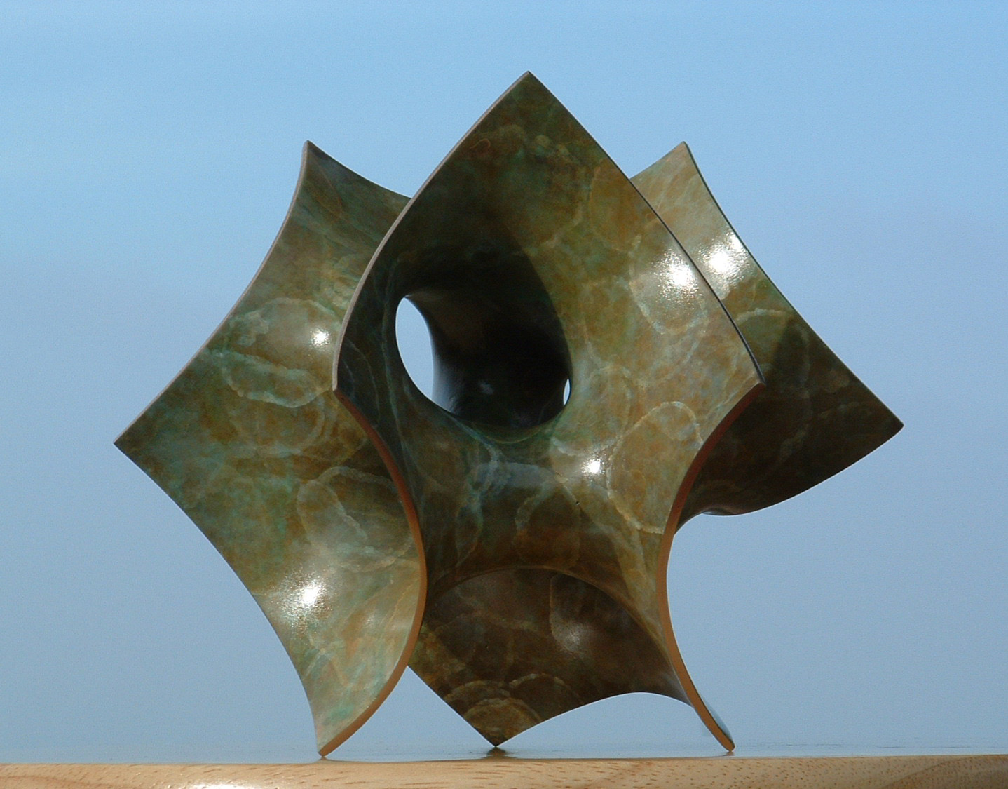

CS 284: Minimal
surfaces
Optimized MVS
Sculpture generator
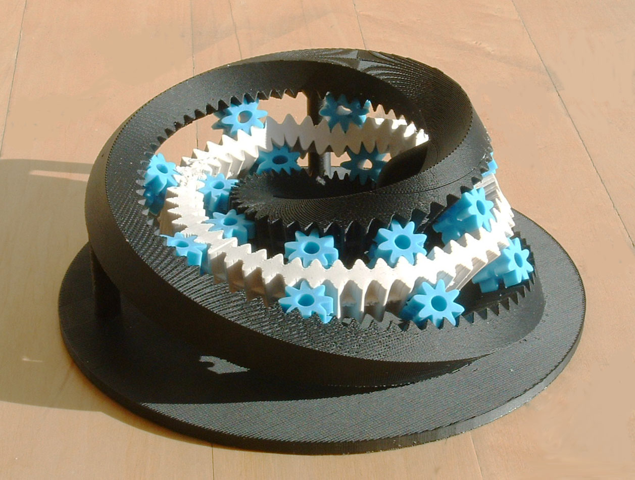
CS 285: Gear generator
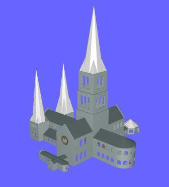
Church builder
L-systems
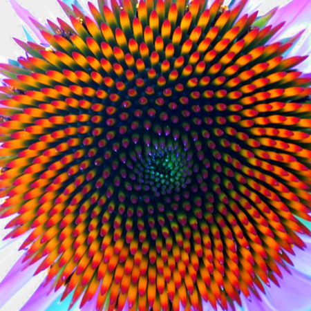
Phyllotaxis
Reading assignments:
Shirley 2nd Ed.: Read Sect. 4.4 - 4.5
Shirley 3rd Ed.: Read Sect. 9.4 - 9.5
Study whatever gives you the needed background information for your project.
CS 184 Course Project: Consult Project Page!
As#12 = PHASE_3:
Intermediate Progress report: Show evidence of the basic core of your project working.
(more details will be forthcoming).
Due Monday May 2, 11pm (worth another 15% of project grade).
Training for Final Exam: Wed. May 4, 10am-11am, 306 Soda Hall.
Final Exam: Friday, May 13, from 8:10 am till 11 am, in the Bechtel Auditorium.
(IEEE may serve some light breakfast from 7:45 till 8:00 in the Bechtel Lounge)
Rules: This is what you will see on the front page:
INSTRUCTIONS ( Read carefully ! )
DO NOT OPEN UNTIL TOLD TO DO SO !
TIME LIMIT: 170 minutes. Maximum number of points: ____.
CLEAN DESKS: No books; no calculators
or other electronic devices; only writing implements
and TWO double-sided sheet
of size 8.5 by 11 inches of your own personal notes.
NO QUESTIONS ! ( They are typically unnecessary and disturb the
other students.)
If any question on the exam appears unclear to you, write down what the
difficulty is
and what assumptions you made to try to solve the problem the way you
understood it.
DO ALL WORK TO BE GRADED ON THESE SHEETS OR THEIR BACKFACES.
NO PEEKING; NO COLLABORATION OF ANY KIND!
I HAVE UNDERSTOOD THESE RULES:
Your
Signature:___________________________________
Think
through the topics covered in this course.
Practice by working through some questions of the posted: Old CS 184 Exams
Prepare one additional sheet of notes to be used during the exam.
Project Demonstrations:
Tuesday and Wednesday, May 10/11, 2011 in 330 Soda Hall
Each group MUST demonstrate their final project.
Sign up for an appropriate time slot -- details on time slots will be posted later.
A sign-up list will be posted on
the instructional web
page: TBA ...
Demos will take place in 330 Soda. Make sure your
demo is ready to run at the start of your assigned demo slot.
Final Project Submission:
Submit your final project report as As#13 -- within one hour after your demo time.
PREVIOUS
< - - - - > CS
184 HOME < - - - - > CURRENT
< - - - - > NEXT
Page Editor: Carlo
H. Séquin