GPCA: Problems & Solutions
This page is designed for a general audience to familiarize with the type of problems that Generalized Principal Component Analysis (GPCA) aims to solve. The intent is that you need not be a researcher in this field in order to understand the background of these techniques and how it can be useful for your own research or application; If you are already an expert in data clustering and machine learning, you can probably skip the background information and read the basic ideas of the solution given by GPCA via a very simple example.
Be aware: Information given here is not meant to be thorough or complete. For a more formal and rigorous introduction to GPCA, you may want to resort to the literature listed in the Publications section.
A. Modeling Data with a Single Subspace
In science and engineering, one of the most common practices is to fit a parametric model to a given set of measurements or sample data. The chosen model can either be geometric (e.g. a plane, a curve, or a surface) or statistical (i.e. a probabilistic distribution). Linear models (e.g., a straight line or a subspace), due to their simplicity, are arguably the most popular and widely-used class of models. The statistical counterpart of linear models is Gaussian distributions.
Given a set of data samples in RD, a standard technique for finding the single best (in the sense of least-square error) subspace of a given dimension is known as Principal Component Analysis (PCA). Without loss of generality, we may assume the data is zero-mean and the subspace to fit is a linear subspace (passing through the origin). Then PCA operates as follows: First collect all the sample points as the column vectors of a matrix; then compute the singular value decomposition of the data matrix; finally the first d singular vectors give a basis of the optimal subspace of dimension d. Furthermore, the sum of squares of all the remaining (D - d) singular values gives the squared error of fitting. As the dimension of the subspace is typically smaller than the dimension of the original space, PCA is often viewed as a method for "dimension reduction."
In a sense, GPCA is about how to generalize the above process to situations in which we need to simultaneous fit multiple subspaces (of possibly different dimensions) to a given data set.
B. Modeling Mixed Data with Multiple Subspaces
B.1. Why Clustering Data?
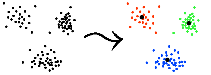
However, in practice, a single linear model has severe limitations for modeling real data. Because the data can be heterogeneous and contain multiple subsets each of which is best fit with a different linear model. Figure 1 shows a simple example where a given set of sample points are clustered around three different centers. Thus, it is more reasonable to fit three, instead of one, linear models to this data set (because each center, as a point, is a zero-dimensional affine subspace).
 Figure 1: Data samples clustered around three different centers (indicated by large black dots). Coloring indicates grouping. |
There is a seemingly "chicken-and-egg" difficulty in modeling mixed (or multi-modal) data such as the one shown in Figure 1: Without knowing which data points belong to which model, how can we estimate each model (in the example, the center of each cluster)? Without knowing the models a priori, how should we assign the data points to different groups?
Traditional approaches typically convert the data cluster problem to a statistical model estimation problem. The resulting solution is often iterative. That is, starting with some initial estimates of the models, one groups the data points to their closest models; once the data are segmented, one re-estimates the models. One then iterates between the above two steps until the solution converges. The representative algorithms are K-means and Expectation Maximization. Source codes of these algorithms can be found in the Sample Code section. In a sense, GPCA deviates from the traditional statistical formulation and seeks new tools from algebraic geometry to resolve the above "chicken-and-egg" difficulty. The resulting algorithm is non-iterative instead.
B.2. Why Subspaces of Higher Dimension?
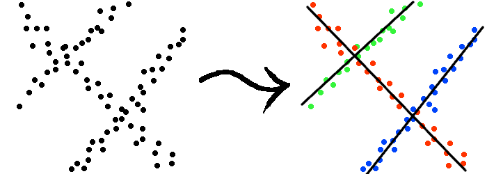
Aforementioned point clusters are too simplistic to describe more complicated geometric structures that the data might have. For instance, as the example shown in Figure 2, the data points might be drawn from a collection of straight lines. Using a point-cluster model, it would be impossible to segment the data set correctly.
 Figure 2: Data samples drawn from three straight lines (indicated by black lines). Coloring indicates grouping. |
Thus, we need to consider a natural generalization of the point-cluster models: the center (or mean) of each cluster is replaced by a subspace (of dimension possibly larger than zero). To allow the model to contain subspaces of higher-dimensions, we can better capture the piecewise linear structures of a given data set and correctly segment the data to the closest subspaces.
B.3. Why Subspaces of Different Dimensions?
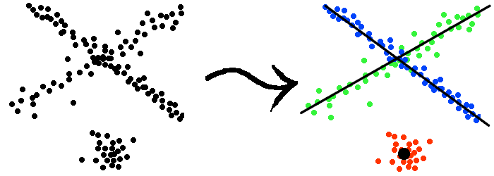
In the above two examples, we have implicitly assumed that the different subsets of the data set are fit with models of the same dimension (they are all points, or lines). However, in practice, real data can be a mixtures of subsets that have different nature and complexity. As the example shown in Figure 3, it is often more reasonable and flexible if we can allow different subsets to be fit with models of different dimensions.
 Figure 3: Data samples drawn from two lines and one point. |
In the above toy examples, the noise in the data is small enough that it is fairly easy to determine the correct types of models for the groups. But in general, selecting the right model and its type can be a very difficult task. In a sense, GPCA tries to solve the general problem: Given a set of (noisy) sample points drawn from a collection of subspaces of possibly different dimensions, determine:
- the number of subspaces,
- the dimensions of the subspaces,
- the optimal basis of each subspace.
C. Methods for Modeling Data with Multiple Subspaces
C.1. Iterative Statistical Methods
If we know the number of subspaces and their dimensions, the problem of fitting multiple subspaces to a data set can be formulated as a statistical model estimation problem. For instance, the data can be assumed to be drawn from a mixture of multiple distributions (e.g., Gaussians). If one seeks the maximum-likelihood estimate of the model, Expectation Maximization (EM) is a typical scheme to maximize the likelihood function of such a mixed distribution. If one seeks the minimax estimate of the model, K-subspaces (a variation of K-means) is a typical scheme to use. Source codes for both schemes can be found in the Sample Code section.
However, as there is no closed-form solution to the maximum-likelihood or minimax estimates, both EM and K-subspaces are iterative schemes and update the solution incrementally. If not initialized properly, both schemes may fail to converge to the globally optimal solution and get stuck to local minima. In addition, both schemes have difficulty in handling situations in which subspaces have different dimensions or the number of subspaces is unknown.