 |
QA<-B T(1 2 1) <-----
QB<-A |
 |
QB<-C S(2 2 2) <-----
QC<-B |
 |
|
University of California EECS Dept, CS Division |
||
|
TA: Laura Downs TA: Jordan Smith |
CS184: Foundations of Computer Graphics |
Prof. Carlo H. Séquin Spring 1998 |
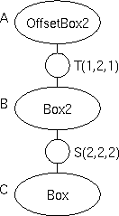
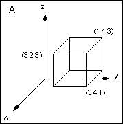
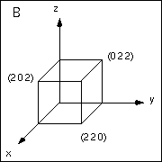
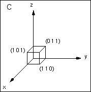
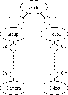
Suppose I have a scene hierarchy as shown at the right. The top level node, or world node, is a translated, scaled box. The bottom level node, or object node, is a box with sides of length and one corner at the origin.
The Qworld<-object transform is the transformation that computes the world coordinates of a point given in object coordinates, i.e. (in column vectors) Qworld<-objectpobject=pworld. In this example, if I take the point, pobject=(0 1 1), on one corner of the original box, and apply the two modeling transforms, the world coordinates of that point, pworld, should be (1 4 3).
In the figure,
the world coordinate system is system A and
the object coordinate system is system C.
Therefore, our world<-object transform will be the
same as the A<-C transform,
i.e.
Qworld<-object=QA<-C,
pobject=pC, and
pworld=pA.
|
QA<-B T(1 2 1) <-----
QB<-A |
|
QB<-C S(2 2 2) <-----
QC<-B |
|
We can't get the QA<-C transform directly, but we
can construct it from the individual transforms in the hierarchy.
We know QA<-B and QB<-C;
QA<-B is the translation, T(1 2 1)
and QB<-C is the scale, S(2 2 2).
Now we have enough information to compute the complete world<-object transform,
Qworld<-objectpobject
=QA<-CpC
=QA<-BQB<-CpC
=T(1 2 1)S(2 2 2)pC
Qworld<-object
=T(1 2 1)S(2 2 2)= |
|
|
= |
|
We also need to know the inverse to that matrix, the Qobject<-world matrix. Rather than invert the Qworld<-object matrix explicitly, we can keep track of the inverse as we move down the hierarchy.
S(1/2 1/2 1/2) T(-1 -2 -1).
The camera transformation computes the coordinates of a point in space relative to the camera. This coordinate system is called the View Reference Coordinates (VRC). This transformation is desirable because camera projections are very easy to compute in this coordinate system.
In the example shown on the right, we have a scene hierarchy containing an object and a camera. Each occurs deep within the hierarchy and is affected by a sequence of transformations. We want to find the camera<-object transformation.
We already know how to find the world<-object transformation that transforms the points in an object's coordinate system into points in the world coordinate system. This is just the concatenation of all of the transforms along the path from the world to the object.
We also know how to compute the inverse of this matrix.
We keep track of both of these matrices as we traverse the scene hierarchy. Each time a transformation is encountered in the traversal, we concatenate it with the Qworld<-object matrix and we concatenate its inverse with the Qobject<-world matrix.
The camera<-object transform is computed from the camera<-world and world<-object transforms.
When we want to render the scene from a particular camera, we first find the world<-camera and camera<-world transforms by traversing the path from the world node to the camera node.
Then, we start at the root node of the scene graph and use the camera<-world transform as the initial modeling transform. Now, all points will be automatically transformed into the camera's frame of reference by the modeling transform.
 The standard camera placement transformation is represented in
GLIDE by the
lookat
transformation.
Although the most common use for this transformation is to place a
camera at one point in space looking at another point in space,
it can also be used to place any object or light in the scene.
The lookat transformation is particularly useful for pointing a
spotlight at something in the scene.
The standard camera placement transformation is represented in
GLIDE by the
lookat
transformation.
Although the most common use for this transformation is to place a
camera at one point in space looking at another point in space,
it can also be used to place any object or light in the scene.
The lookat transformation is particularly useful for pointing a
spotlight at something in the scene.
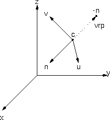
The lookat transformation specifies a new coordinate system, (u,v,n) within the current system by
In order to compute the transformation matrix for the lookat transform, we must first find the orthonormal coordinate axes (u,v,n) and the origin c.
Now that we have the necessary information: the origin, c, and the coordinate axes, (u,v,n), we can compute the lookat transformation, Qlookat. The matrix, Qlookat, will transform points in the camera's or object's system into the world system just like any other modeling transform.
Let's call puvn=(pu pv pn) and pxyz=(px py pz)
pxyz
= T(c) Qxyz<-uvn puvn
= T(c)
|
|
|
so we get
Qlookat
= T(c) Qxyz<-uvn
where
Qxyz<-uvn =
|
|
and Quvn<-xyz = |
|
We also need to find Qlookat-1, which we can do in a straightforward fashion:
T(c) Qxyz<-uvn)-1
= Qxyz<-uvn-1 T(c)-1
= Qxyz<-uvnT T(c)-1
= Quvn<-xyz T(-c)
We start out with some arbitrary view frustum or parallelepiped as defined by the frustum parameter in the GLIDE camera statement. We need to transform this volume into a canonical volume so that we can clip our polygons against standard clipping bounds and apply a standard projection to their vertices. The normalizing operation is slightly different for the parallel and perspective projections.
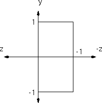
| We start with a parallelepiped as defined by the frustum, (xmin, ymin, zmin) (xmax, ymax, zmax). The (xmin, ymin) and (xmax, ymax) pairs describe the rectangular cross-section in the z=-1 plane. The zmin and zmax values describe the back and front planes. The direction of projection (dop) is from the origin to the midpoint of that rectangle. | 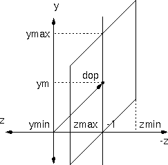 | |||||||||||||||||
First we have to shear the volume so that all of the boundaries are
axially aligned and the dop lies along the -z-axis.
Let ym = (ymin+ymax)/2
and xm = (xmin+xmax)/2.
Then our shear matrix is:
|
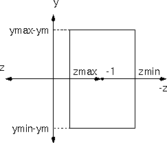 | |||||||||||||||||
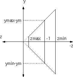
Next, we translate the volume so that the front clipping plane
corresponds to the xy-plane.
This involves just a translation by -zmax in z,
T(0,0,-zmax)
|
||||||||||||||||||
|
Finally, we scale the volume non-uniformly to match the bounds: -1 <= y <= 1, -1 <= z <= 0. S(1/(xmax-xm), 1/(ymax-ym), 1/(zmax-zmin))
|
 |
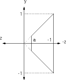
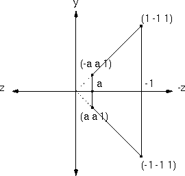
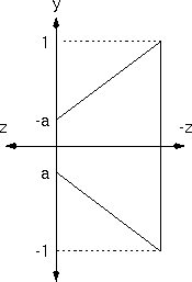
| We start with a frustum as defined by the frustum, (xmin, ymin, zmin) (xmax, ymax, zmax). The (xmin, ymin) and (xmax, ymax) pairs describe the rectangular cross-section in the z=-1 plane. The zmin and zmax values describe the back and front planes. | 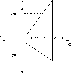 | |||||||||||||||||
First we have to shear the volume so that the center of the frustum
lies along the -z-axis.
Let ym = (ymin+ymax)/2
and xm = (xmin+xmax)/2.
Then our shear matrix is:
|
 | |||||||||||||||||
|
Then, we scale the volume non-uniformly to match the bounds: z <= y <= -z, -1 <= z <= a, S(1/(xmax-xm), 1/(ymax-ym), 1)Then we scale the whole frustum uniformly by -1/zmin so that the back clipping plane lies in the z=-1 plane. S(-1/zmin, -1/zmin, -1/zmin)which gives us a value for a of a = -zmax/zmin. |
 |
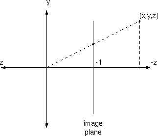
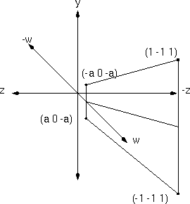
Now, we are in a normalized space oriented with the camera sitting at the origin, pointing down the -z-axis. If we take any point in the scene, say p=(px,p,y,pz), we want to find the projection of that point onto the image plane, z=-1. This projection is the intersection of the ray starting at the origin and passing through the point, p.
We can find the coordinates of that point using an old trick from geometry, similar triangles. The triangle shown in dashed lines in the picture has height=py and width=-pz. The triangle formed by the projection ray, the image plane and the -z-axis has width=1. So, by similar triangles, the height of that triangle is py/(-pz).
This value, py/(-pz), is the projected y-value of the point. Similarly, the projected x-value is px/(-pz). This non-linear operation can be performed in homogeneous coordinates by allowing a w-value that is not 1. We simply apply this operation: w' = -z
Unfortunately, this operation is not invertible because the
new z and w values are linearly dependent.
Also, after the homogeneous normalization (division by w) has
been applied, all of the z values will be -1.
In order to maintain z ordering, we need to transform z
to some other value.
We will use the value:
The transformation matrix that applies this perspective transformation is:
| Qproj<-vrc = |
|
| Qproj<-vrc-1 = |
|
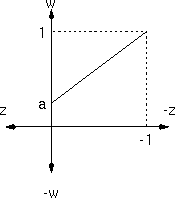
 Visualizing the effect of a 4D transformation is pretty tough, so here
is an analogous 3D transformation.
The x-coordinate in our regular space is transformed just like
the y-coordinate is here.
Visualizing the effect of a 4D transformation is pretty tough, so here
is an analogous 3D transformation.
The x-coordinate in our regular space is transformed just like
the y-coordinate is here.
Here we have a homogeneous 2D space with no x-coordinate.
The figure to the right shows the normalized frustum in the w=1
plane just before the perspective transformation (warp).
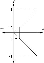
The figures below show the (y,z) view volume after its
perspective warp.
| The transformed homogeneous plane viewed along the y-axis | The transformed homogeneous plane viewed along the z-axis | The transformed homogeneous plane viewed along the w-axis | The transformed homogeneous (y,z,w) plane |
 |
 |
 |
 |
For a parallel projection: Once we are in the normalized half-space, a plane is front facing if the z-component of the normal is positive, i.e. c > 0.
For a perspective projection: Once we are in the normalized frustum, a plane is front facing (its normal points towards the camera/origin) if d > 0. After we have applied the perspective warp to the plane equation (Qproj<-vrc-1)TN, we have a new value c' = -(1+a)d/a. So, if this value is positive, (c' > 0), then we have -(1+a)d/a > 0 and thus d > 0.
Therefore, we only have to check the value for c in the final plane equation after perspective warp to determine whether a plane faces the camera and we do not have to homogenize the plane equation. Homogenizing the plane equation can reverse the direction of the normal and lead to incorrect culling.
In the parallel case, w=1, so the bounds become:
In the perspective case, w=-z, so the x and y bounds become:
Clipping against these planes is nearly as easy as clipping against
the axially aligned planes. For example, suppose we are clipping two
points,
p1=(x1,y1,z1)
and
p2=(x2,y2,z2)
against the x=w plane.
We have already determined that the two points lie on opposite sides
of the plane (i.e. for one of them x>w and for the other x<w).
We want to find the intersection point:
pt = p1 + t(p2 - p1)
with xt=wt.
This gives us the formula
Because this parameter, t is computed from coordinates that are all linearly derived from the initial, object space, coordinates of the two points, it can be used to correctly compute interpolated values along the edges of the polygon. If the points were normalized (divided through by w) before the clip, the parameter value would not be the correct value. For example, consider the midpoint in screen space of a line that starts very close to the viewer and ends very far away. The visual midpoint will be much closer to the near end of the line than to the far end of the line in object space although the homogenized parameter value would be t=0.5.
Questions:
Last modified: Tue Mar 31 19:51:50 1998