CS 184: COMPUTER GRAPHICS
Feedback Results:
Most say the assignment are interesting !
The reported hours/week range from 3 to 48 !!
Peak is around 10, median around 12, mean about 14.
Some consider 6hrs "heavy" and 10hrs "too much."
Some report 12 hrs and consider this "light", others 16 hrs and consider this "OK"
50%-50% split on doing assignments alone, versus in pairs.
[ Comments:
This is a 4-unit course. The CS norm is that this should involve about 12hrs of work outside lectures.
If you were unfamiliar with C++, then this course would be an additional 1-2 unit course, adding 3-6 more hours.
We will extend the time spans for the next assignments by a couple of days.
On AS#6 you get the option of doing it alone or as a pair.]
Lecture speed seems to be about OK, perhaps bit on the fast side since we have started ray-tracing.
Many students would like to see more demos, visualizations, cool pictures,
but also more examples, more explanations, more details on C++ and OpenGL.
[ I would like to have a 3rd lecture each week !
C++, OpenGl, coding issues are deliberately reserved for the discussion sections.
You can also find many cool pictures yourself on Google_Images; e.g., search "ray-tracing".]
PREVIOUS
< - - - - > CS
184 HOME < - - - - > CURRENT
< - - - - > NEXT
Lecture #12 -- Wed 3/4/2009.
YOU are producing some cool pictures already !
Samples from the Hall of Fame of CS184_Spring 2009:
Adrian Marple: http://inst.cs.berkeley.edu/~cs184-bm/as2.html -- sordfish - ant-eater?
Mathew Carlberg: http://inst.cs.berkeley.edu/~cs184-bl/assignment2.html -- crab - shark
Zelam Ngo and Partner Scott "ai" Hoag: http://inst.cs.berkeley.edu/~cs184-bb/assignment3.html -- "wink-wink"
Reid Hironaga: http://inst.cs.berkeley.edu/~cs184-bq/assignment4.htm
-- circling lights
Schedule Preview:
AS#5 due Sunday 3/8, 11pm
Take-Home-Exam: from Monday 3/9 till Wednesday 3/11 class time.
AS#6 due Tuesday 3/17, 11pm
(may be done in pairs).
AS#7 (roller coaster and "flying camera") due after Spring break, WED
4/1, 11pm
In-class Mid-term-Exam: WED 4/8, 2:40-4:00pm
Eficiency Aspect: Exploiting Locality and Coherence [10.9] (cont.)
Ray - Triangle Intersection
How do we know which side of the triangle we are hitting ?
Face normals point "outwards" from solids; contour vertex sequence is seen in CCW order.
Hierarchical Bounding Boxes [10.9.2; Fig. 10.19]
Flatten scene into a "sea of primitives"; determine the centroid for each primitive, and the
overall bounding box around the whole scene.
Pick the longest axis of this bounding box, and sort all centroids
along this axis; then split the whole population at the median into two
halves of equal magnitude.
Recursively continue this splitting process for the two halves.
Traverse Bbox hierarchy recursively from the root.
Uniform Spatial Subdivision [10.9.3; Fig. 10.20]
Flatten scene into a "sea of primitives."
Fill the overall bounding box around the whole scene with a uniform 3D
grid (about a thousand grid cells for a million triangles).
Link each primitive to all the the cells that it overlaps.
A ray traverses the scene going from cell to cell (starting from the
eye); for each cell, test all the primitives linked to it (keep range
of "t" to keep ray in cell).
Binary Space Partitioning [10.9.4; Fig. 10.24]
As for the Hierarchical Bounding Box scheme, partition space recursively into a balanced binary tree.
At each node we keep the equation of the splitting plane
and pointers to the two subtrees on either side of it, which
contain all objects that touch that space;
thus objects that straddle the splitting plane will be linked to both subtrees.
A ray would first test the subtree on the side of the plane where it
originates, and if there is no hit test the contents of the other side
of the plane.
[ see Shirley Ch. 8.1 for a BSP tree in the context of hidden surface
elimination; here we split along the arbitary planes defined by the
individual polygons ]
Mixed, Structural, Adaptive, Partitioning
The techniques described above can be mixed and combined to best fit a scene of a special type.
For instance, if the scene has a few complicated objects slowly moving
against one another, separate partitionings could be done withing the
bounding boxes of every object.
If the density of primitives varies strongly within the whole scene or
withing any such object bounding box, then an adaptive
octree-based space partitioning could be used.
Rays interrogate the Bboxes of the logical scene hierarchy as in the Hierarchical Bounding Box scheme,
and then inside the leaf boxes of the scene they proceed in a
spatially ordered manner as in one of the space partitioning schemes.
How Can We Describe 3D Objects ?
Voxels
and Octree:
Concept: sample space regularly;
determine whether the sample falls inside or outside of object, e.g., by an implicit function;
"turn on" inside voxels.
Efficient encoding required: e.g., quadtree in 2D, octree in 3D.
Good for representing: MRI-scans, CAT-scans, brains, sponge-like objects,
clouds, ...
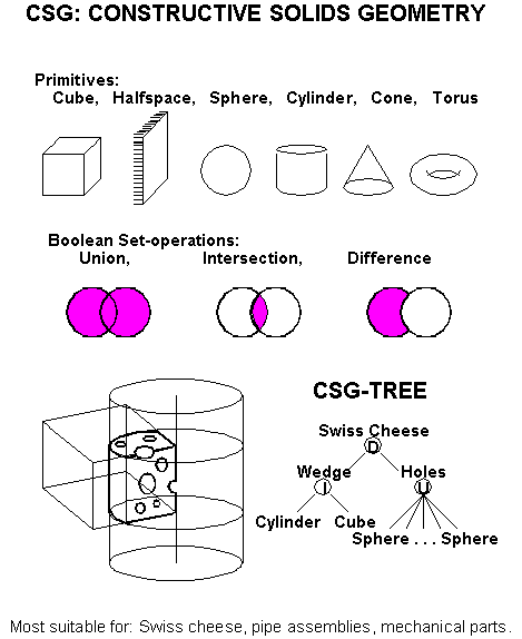
CSG
and Boolean set operations:
CSG = Constructive Solid Geometry.
The object is composed from (overlaping) primitive geometric shapes,
typically: cubes, halfspaces, spheres, cylinders, cones, tori, ...
e.g., a "Sausage" = bent cylinder plus spherical end-caps (show 2D
composite).
Good for representing: mechanical parts, Swiss cheese, results of solid
modeling operations, ...
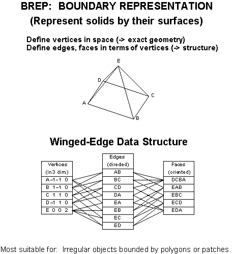
B-rep
and winged-edge data structure:
Tessallate surface; describe polyhedral objects via vertices, edges, faces;
or "meshes" (triangle strips, fans) that use a more efficient encoding
of the connectivity.
Good for representing: polyhedral objects with odd angles, tessellated
parametric surfaces, ...
Procedural modeling:
A program fragment creates the vertices and faces and their connectivity,
or, alternatively, the instance calls to CSG primitives,
or a collection of "inside" voxels,
or an implicit function, which may then be converted to one of the
above representations.
Good for representing: parameterized, iterated objects;
e.g., gearwheels, fractal mountains, trees, geometrical
sculpture, ...
Commonly used generic procedures: Sweeps:
(axial, rotational, or along an arbitrary path).
For "Sausage": Sweep a circle through space along a curve. Start small
for front-cap;
keep constant through main part of sausage; taper down to zero for
end cap.
Good for representing: pipes, sausages, moldings, rotationally symmetrical
(turned) objects, geometrical
sculpture, ...
Another example: Subdivision Surfaces (discussed later in the
course).
3D B-Rep Modeling Primitives and "Winged-Edge" Data Structure
[13.1-13.2].
Faces - again, described efficiently by an ordered sequence of vertices; -- but "should" be planar.
We need to find their plane equation; needed for calculation
of illumination:
Martin
Newell's plane equation formula:
Plane normal components are in same ratio as shadow of polygon on the
three coord planes.
Each shadow area is computed as 2D projection as sum of trapezoids
(x1-x2)(y1+y2)/2.
Form the sum of all such expressions around the contour; do it for
all 3 projections.
Reading Assignments:
Study: ( i.e., try to understand fully, so that you can answer
questions
on an exam):
Shirley, 2nd Ed: Ch 10, Ch 13.1-13.2
Skim:
Shirley, 2nd Ed: Ch 8.1
Programming Assignment 5: To be done individually; due (electronically submitted) before Sunday 3/8, 11pm.
NEWS: Sunday 5pm:
Don't break your back over refraction! (The test image seems to have a flaw in it in that respect).
We will treat refraction as extra credit, if you already did it, but won't penalize you if you have trouble with it!
Take-Home-Exam: from Monday 3/9 till Wednesday 3/11 start of class.
Programming Assignment 6: due (electronically submitted) before Tuesday 3/17, 11pm <== THIS ASSIGNMENT CAN BE DONE IN PAIRS !
PREVIOUS
< - - - - > CS
184 HOME < - - - - > CURRENT
< - - - - > NEXT