CS 184: COMPUTER GRAPHICS
PREVIOUS
< - - - - > CS
184 HOME < - - - - > CURRENT
< - - - - > NEXT
Lecture #28 -- Th: 12/09, 2004
Comparing Different Rendering Paradigms
The Classical Rendering Pipeline (object space):
Geometric Model
Camera Placement
Perspective Projection
Visibility Calculation
Illumination
Rasterization
Display
Ray-Tracing Pipeline (image space):
Geometric Model
Camera Placement
Ray Casting / Visibility Calculation / Rasterization ==> all in
one !
Light-source Probing
Radiosity Pipeline (object space):
Geometric Model
Global Illumination ==> becomes part of the scene !
Camera Placement
Perspective Projection
Visibility Calculation
Rasterization
Display
Review: Radiosity Rendering
In the simplest case we assume all the surfaces are perfectly diffuse reflectors.
Thus the apparent brightness of a surface is independent of viewer
position.
However, large (flat) polygons can still have non-uniform brightness
because of non-uniform illumination.
We now consider indirect illumination by other illuminated and diffusely
reflecting surfaces.
For this, we break up large surfaces into small flat polygons (patches)
over which we can assume the brightness to be constant.
Once all the patches have been assigned their brightness (color) values,
we can render the scene from any viewpoint.
To calculate the amount of diffuse illumination that gets passed from
one patch to another, we need to know the form factor between them.
This form factor describes how well the two patches can see
one another (depends on distance, relative orientation, occluders between
them).
Once we have determined all these purely geometrical form factors,
we could set up a system of p linear equations in the radiosity of the
p patches.
Solving this system with a direct method (e.g. Gaussian elimination)
is not practical, if there are thousands or millions of patches.
But we can exploit the fact that most of the form factors are typically
zero, since many pairs of patches cannot send much light to each other.
Thus we can apply an iterative approach:
First consider only the light directly emitted by the active light sources.
Then add the light that results from only a single reflection on
any surface from the source lights.
Next add the light that has seen two reflections, and so on ...
The process is stopped locally whenever the additional contributions fall
below some desired level of accuracy.
Two-pass Method
One way to combine the best capabilities of radiosity-based rendering
(indirect lighting by diffuse-diffuse interreflections)
and of ray-tracing (specular reflections, translucency), is
to use a two-pass method.
The first pass is a radiosity-like algorithm that creates an approximate
global illumination solution.
In the second pass this approximation is rendered using an optimized
Monte Carlo ray tracer (statistical sampling).
This scheme works very well for modest scenes.
But for models with millions of polygons, procedural objects, and many
glossy reflections, the rendering costs rise steeply,
mainly because storing illumination within a tessellated representation
of the geometry uses too much memory.
Photon Mapping
The above approach can be improved, if a photon map is used to represent
the overall illumination within a model.
This photon
map is created by emitting a large number of photons from the light
sources into the scene.
Each photon is traced through the scene, and when it hits a non-specular
surface, it is stored in the photon map.
These photons stored within the model approximate the incoming light
flux at the various surfaces.
This photon map can then be used to produce radiance estimates at any
given surface position.
The method can be further improved by using two photon maps:
A high-resolution photon map represents caustics (spots where
light is concentrated by lensing effects) to be visualized directly;
and a global photon map of lower resolution serves to reduce
the number of reflections that need to be traced
and to generate optimized sampling directions in the Monte Carlo ray
tracer (to increase its efficiency).
Photon mapping makes it possible to efficiently simulate global illumination
in complex scenes, even when they include participating media.
Example: A
simple museum scene rendered with photon mapping.
Note the caustic below the glass sphere, the glossy reflections, and
the overall quality of the global illumination.
Source: http://graphics.stanford.edu/~henrik/papers/ewr7/ewr7.html
Background: Realistic
Image Synthesis Using Photon Mapping by Henrik Wann Jensen
--- from here on : FOR ENRICHMENT ONLY -- NOT ON FINAL EXAM ---
Participating Media
The intensity and color of light rays may not only be changed when they
interact with discrete surfaces.
When light
rays pass through media that are not completely transparent (water,
vapor, fog, smoke, colored glass ...),
the interaction with these media happens along the whole path,
and the resulting effect increases exponentially with the length of
the path.
(If the effect is small enough, a linear approximation can be used.)
When scenes contain smoke or dust, it may be necessary to take into account
also the scattering
of light as it passes through the media.
This involves solving the radiative transport equation (an integro-differential
equation),
which is more complicated than the traditional rendering equation solved
by global illumination algorithms.
The photon map method (see below) is quite good at simulating light
scattering in participating media.
- ---
So far all scenes have been modeled with B-reps ...
but what do we do if we have voxel data ?
Volume Rendering
If we want to render the boundary of a sampled 3D scalar field (e.g., MRI
data), we could convert the voxel data into a B-rep,
by using an algorithm called Marching
Cubes (interpolate
surface between sample points), and then use a traditional rendering
pipeline.
Volume rendering is a technique for directly displaying sampled 3D data without
first fitting geometric primitives to the samples.
In one approach, surface shading calculations are performed at every
voxel using local gradient vectors to determine surface normals.
In a separate step, surface classification operators are applied to
obtain a partial opacity for every voxel,
so that contour surfaces of constant densities or region boundary surfaces
can be extracted.
The resulting colors and opacities are composited from back to front
along the viewing rays to form an image.
(Notice connection to transparency lecture!)
The goal is to develop algorithms for displaying this sort of data
that are efficient and accurate, so that one can hope to obtain
photorealistic real-time volume renderings of large scientific,
engineering, and medical datasets on affordable noncustom hardware.
(like nested bodies of "jello" of different colors and densities).
Example: Scull
and Brain
Source: http://graphics.stanford.edu/projects/volume/
An ideal volume rendering algorithm would reconstruct a continuous function
in 3D, transform this 3D function into screen space,
and then evaluate opacity integrals along line-of-sights.
In 1989, Westover introduced splatting for interactive volume
rendering, which approximates this procedure.
Splatting algorithms interpret volume data as a set of particles
that are absorbing and emitting light.
Line integrals are precomputed across each particle separately, resulting
in "footprint" functions.
Each footprint spreads its contribution in the image plane.
These contributions are composited back to front into the final image.
Background: EWA
(elliptical weighted average) Volume Splatting
Point-based Rendering
This is a recent development rapidly gaining poularity.
The whole scene is simply described as a cloud of varying density of sampled data points.
When rendering a pixel representing a particular location, a suitable neighbor hood of sample points
is interrogated, an averaged surface normal is calculated and their colors are combined to produce a small facet
that can be suitably illuminated with the available light sources, so that the pixel color can be determined.
see: PointShop3D Example
Reference: PointShop 3D
Reality Acquisition
So far we have dealt with the rendering of synthetically generated scenes.
Often people would like to capture an existing scene (a complex 3D
object, the interior of a house, a landscape ...)
and create a model from it that can then be rendered from arbitrary
viewpoints and with different illuminations.
One approach is to use a 3D scanner that takes an "image" by
sampling the scene like a ray-casting machine,
but which also returns for each pixel a distance from the scanner.
This collection of 3D points is then converted into a geometrical model,
by connecting neighboring sample dots (or a subset thereof) into 3D
meshes.
Color information can be associated with all vertices, or overlaid
as a texture taken from a visual image of the scene.
This all requires quite a bit of work, but it results in a traditional
B-rep model that can be rendered with classical techniques.
Challenges are: to combine the point clouds taken from different
directions into one properly registered data set,
to reduce the meshes to just the "right number" of vertices, and to
clean up the "holes" along silhouette edges
Image-based Rendering
Unlike the shape capture process above that can be used with a traditional
rendering pipeline,
the following approaches do not rely on a geometric representation.
This alternative approach to reality capture starts with many 2D
images and
then creates new images for different viewpoints by cleverly combining
information from these images.
In one approach,
two "stereo pictures" are taken of a scene from two camera locations
that are not too far apart.
Manually, or with computer vision techniques, correspondence is
established between key points in the two renderings.
By analyzing the differences of their relative positions in the two
images, one can extract 3D depth information.
Thus groups of pixels in the both images can be annotated with a distance
from the camera that took them.
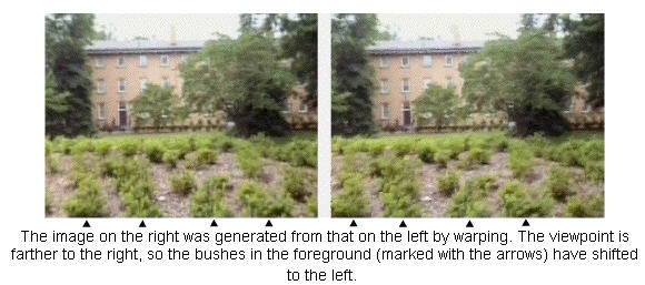
This basic approach can be extended to many different pictures from
different camera locations.
The depth annotation establishes an implicit 3D database of the geometry
of the model object or scene.
To produce a new image from a new camera location, one selects
images taken from nearby locations
and suitably shifts or "shears" the pixel positions according to their
depth and the difference in camera locations.
The information from the various nearby images is then combined in
a weighted manner,
where closer camera positions or cameras that see a surface under a
steeper angle are given more weight.
With additional clever processing, information missing in one image
(e.g., because it is hidden behind a telephone pole)
can be obtained from another image taken from a different angle,
or can even be procedurally generated by extending nearby texture patterns.
Example 1: Stereo
from a single source:
A depth-annotated image of a 3D object, rendered from two different
camera positions.
Source http://graphics.lcs.mit.edu/~mcmillan/IBRpanel/slide06.html
Example 2: Warped
image from a neighboring position:
Background: UNC Image-Based Rendering
Light Field Rendering and the Lumigraph
These methods use another way to store the information acquired from a
visual capture of an object.
If one knew the complete plenoptic function (all the photons
traveling in all directions at all points in space surrounding an object),
i.e., the visual information that is emitted from the object in all
directions into the space surrounding it,
then one could reconstruct perfectly any arbitrary view of this object
from any view point in this space.
As an approximation, one captures many renderings from many locations
(often lying on a regular array of positions and directions),
ideally, all around the given model object, but sometimes just from
one dominant side.
This information is then captured in a 4D sampled function (2D
array of locations, with 2D sub arrays of directions).
One practical solution is to organize and index this information (about
all possible light rays in all possible directions)
by defining the rays by their intercept coordinates (s,t) and (u,v)
of two points lying on two parallel planes.
The technique is applicable to both synthetic and real worlds, i.e.
objects they may be rendered or scanned.
Creating a light field from a set of images corresponds to inserting
2D slices into the 4D light field representation.
Once a light field has been created, new views may be constructed by
extracting 2D slices in appropriate directions.
Technical challenges:
finding appropriate parameterizations for the light field,
creating light fields efficiently and with proper prefiltering,
displaying them at interactive rates and with proper resampling,
and compressing them to reduce memory use.
-
"Light Field Rendering":
Example: Image
shows (at left) how a 4D light field can be parameterized by the
intersection of lines with two planes in space.
At center is a portion of the array of images that constitute the entire
light field. A single image is extracted and shown at right.
Source: http://graphics.stanford.edu/projects/lightfield/
Background: Light
Field Rendering by Marc Levoy and Pat Hanrahan
Demos:
The light field viewer demo is in S:\bmrt\lightfield
go to that directory with the command prompt and use these commands
to view:
lifview dragon32.lif
lifview buddha4c.lif
up and down arrows zoom in and out....
You can also download it from:
Q:\sequin\public_html\CS184\DEMOS\lifview dragon32.lif
Q:\sequin\public_html\CS184\DEMOS\lifview buddha4c.lif
"The Lumigraph":
Example: The reconstruction of a desired image from given
image information: diagram1
and diagram2
Source: http://research.microsoft.com/MSRSIGGRAPH/96/Lumigraph.htm
Background: Unstructured
Lumigraph Rendering
-
Fire, Smoke, Clouds, Water, Mud, ...
-
Clothes, Silk, Knitwear ...
-
Human Skin, Faces.
Caveat:
Of course the above presentations are much too short and superficial.
The goal is to make you aware that there are many other rendering methods
beyond the ones we have covered in this course.
You can learn more about these in some of our graduate courses, --
e.g. CS294-? (CS283): "Graduate Computer Graphics".
Here I provide you at least with some references and some keywords
that will lead you to further information on the Web.
HOWEVER:
Everything that you have learned in CS184 (scene hierarchies, transformations, dealing with pixels ...)
still very much applies in all these more advanced settings!
Project Deadline is Monday, December 13, 7:59pm. -- FOR EVERYBODY !
(Every day late: -40 points)
Sign up for a project demo slot! http://inst.eecs.berkeley.edu/~cs184/Fa2004/signup/
Make sure your demo is ready to run at the beginning of your assigned demo slot;
have your score sheet properly filled in (including your names and logins).
Final Exam
Thursday, December 16, 8am - 11am, 306 and 310 Soda Hall (not LeConte!)
Review
the midterm topics list.
Think
through the additional topics list for the final exam.
Prepare one additional sheet of notes to be used during the exam.
The TA's have offered to hold a review session:
MONDAY evening, December 13, 2004, 8:30pm-10pm.
PREVIOUS
< - - - - > CS
184 HOME < - - - - > CURRENT
< - - - - > NEXT
Page Editor: Carlo H. Séquin