CS 184: COMPUTER GRAPHICS

PREVIOUS < - - - - > CS 184 HOME < - - - - > CURRENT < - - - - > NEXT

Veterans' Day -- Th: 11/11, 2004

Lecture #22 -- Tue: 11/16, 2004

Return and discuss Midterm Exam

In the first 2/3 of this class you have been given a detailed view of the inside of a typical graphics pipeline
and should have gained an understanding of many basic computer graphics algorithms.

In the last third of this class, you will get a glimpse of some other graphics tool that are out there,
and learn how to deal with them from a user's point of view.
In particular, in assignment #9 you will learn how to use lights, surface parameter specifications
and texturing to turn "bare" geometry into interesting computer graphics images.
And int the final course project you will have a chance to focus on modeling
and to use some of the power in SLIDE to make dynamic, interactive objects.

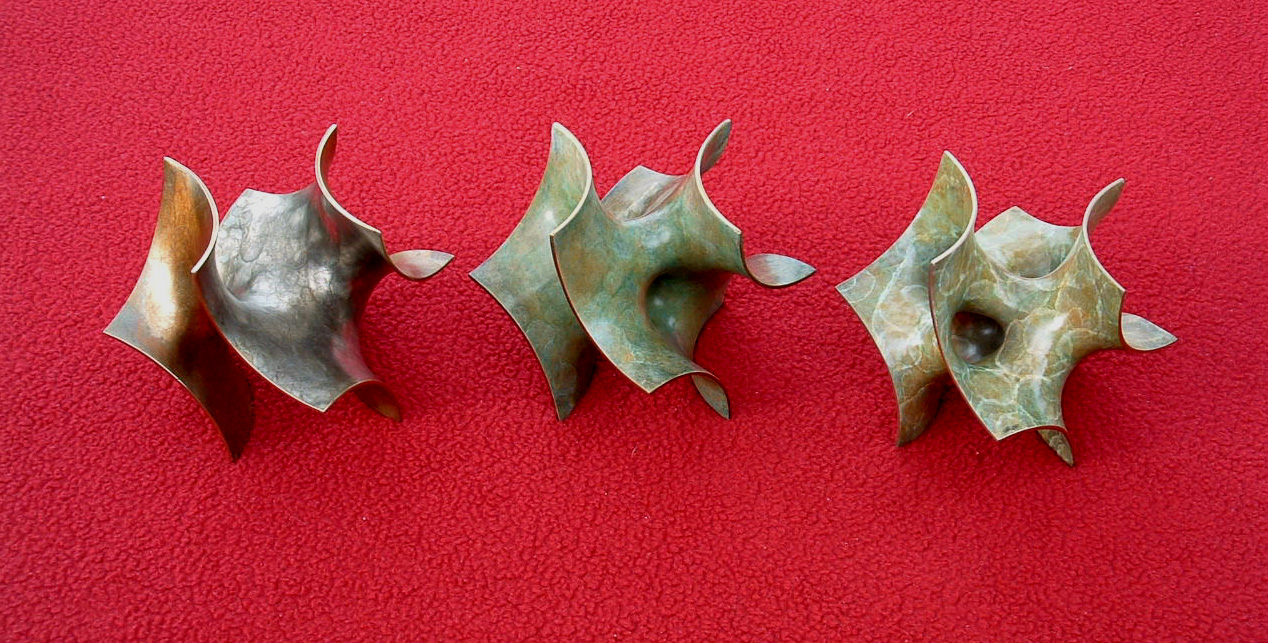
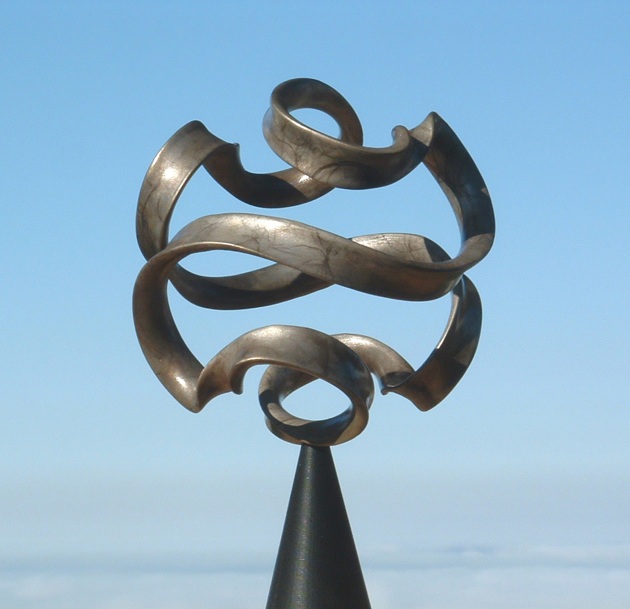
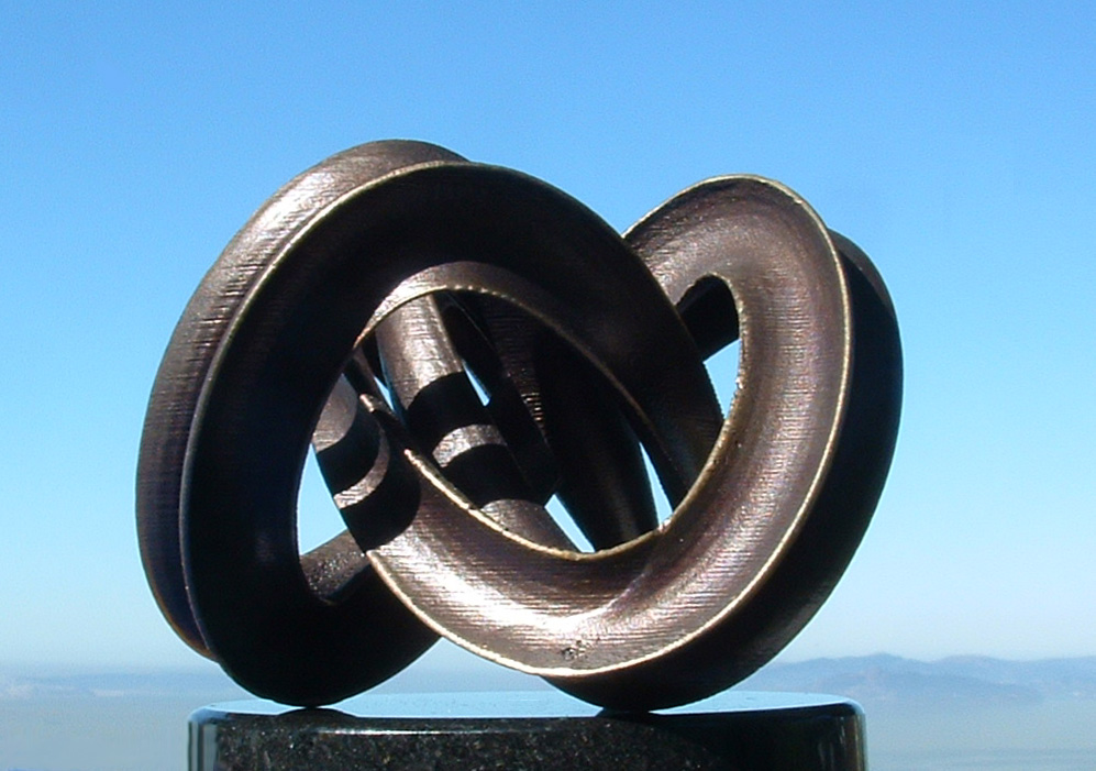
Assignment #9

Starting form some "bare" pieces of geometry, you are asked to use suitable surface parameters,
texturing, and sophisticated lighting, to present these objects as attractive large-scale sculptures that
could be found in a public place or as precious miniatures that could be found in a museum display.
Here are some examples, how I show off some of my sculpture models:

"Totem 3" (September 2004) - Bronze, 13" tall (outdoor setting)
"Volution's Evolution" (August 2004) - 3 bronzes, 5" cube (museum setting)
"K12 Graph on Genus-6 Surface" (June 2004) - 3D print, painted, 5"diam. (table-top setting)
"Genus-6 Kandinsky Surface" (June 2004) - 3D print, painted, 5"diam. (neutral background to enhance colors on sculpture)
"Maloja" (August 2003) - Bronze, 4.2" diam. (outdoor setting)
"Infinit Duality" (August 2003) - another view - Bronze, 3" diam. (outdoor setting)
"3 Congruent Hamiltonian Paths on 4D Cross Polytope" (May 2004) - 3D-Print, 5" diam. (dark background -> night setting ?)

You need to add just a minimum amount of extra geometry to the given forms:
-- a scaled cube, cylinder, or cone as a pedestal,
-- some polygons to give a ground plane or a table top,
-- and perhaps some background or some walls.
These additional elements can easily be textured,
while not all provided sculpture forms lend themselves readily to texturing.

The key purpose of assignment #9 then is for you to explore - from a user's point of view -
several other rendering techniques that go beyond what can be done in SLIDE.
At a later time, we will go into more details how these rendering techniques work.
For now you should just obtain an understanding about the basic paradigms involved,
so that you can make reasonable judgements on how to set the various parameters.
See on-line notes !

Texture Mapping:
Two more scalar values need to be stored at each vertex (s,t).
Rendering textures is easy: Bilinear interpolation of the texture coordinates s,t.
Modeling is more difficult: How to assign texture coordinates to avoid pattern discontinuities?
(see Ch 9-9.4; Color Plate 6 in Angel, 2nd Ed.)
(see Ch 7-7.8; Figure 7.15 in Angel, 3rd Ed.)
(see also Color Plates II.35 - II.37 in Foley et.al.)

3D (Solid) Texture Generation:
To depict realistically 3D objects made from wood or stone,
the patterns shown on adjacent surface polygons have to match in such a way as to imply
a coherent 3D pattern that fills the volume inside the B-rep (e.g., wood grain).
We thus need to define a function that generates a 3-dimensional texture field (s,t,r)
-- fortunately, there are many preprogrammed shaders out there, so you do not have to write this function.
During rendering, the (x,y,z) coordinates on the B-rep (bilinearly interpolated on each polygon)
are then used as arguments to generate texture values at the desired pixel locations.
(see Ch 7.6.5; in Angel, 3rd Ed.)
(see also Color Plates IV.21; Ch 20.1.2 in Foley et.al.)

Area Light Sources:
Some geometry that actively emits light over its surface.
SLIDE approximation: An array of spot lights covering the surface
and sending light primarily in the direction of the surface normal.

Ray-tracing:
Another rendering paradigm:
"What do we see when we shoot a sampling ray through each pixel?"
(see Ch 6.10.1; Color Plate 23 in Angel, 2nd Ed.)
(see Ch 13.2-13.3; Color Plate 23 in Angel, 3rd Ed.)
(see also Color Plates III.10 - III.16 in Foley et.al.)

Antialising:
Reduce the bad effects of sampling
by taking more samples (oversampling) and then averaging the results.
(see Ch 9.7.4; Color Plate 2 in Angel, 2nd Ed.)
(see Ch 7.9.4; Color Plates II.35 - II.37 in Angel, 3rd Ed.)

Radiosity:
Yet another rendering paradigm:
"How do the photons from the light source(s) travel around the scene?"
(see Ch 6.10.2; Color Plate 24 in Angel, 2nd Ed.)
(see Ch 6.10, Ch 13.5; Color Plate 24 in Angel, 3rd Ed.)
(see also Color Plates III.17 - III.28 in Foley et.al.)

Photon Mapping:
is a higly efficient, statistical technique for simulating Global Illumination. It does the work in two phases: First it shoots photons statistically proportional to the intensities of the given light sources and records their landing sites, to get a rough idea of the illumination present on the various surfaces. In the second phase, Ray-Tracing is used figure out what can be seen and what the direct illumination is on those surfaces. For the indirect illumination from the walls and from other objects, the stored Photon Map is suitably queried and interpolated.

Fog:
A special (simple) case of Volume Rendering:
Attenuate and discolor visible information that comes from further away.
(see Ch 9.7.6; Color Plate 8 in Angel, 2nd Ed.)
(see Ch 7.9.6; Color Plate 23 in Angel, 3rd Ed.)

Reading Assignment:

Study: 2ndEd: Ch 6.1-6.5, Ch 6.10, Ch 9-9.7
Study: 3rdEd: Ch 6.1-6.5, Ch 6.10, Ch 7.5-7.9, Ch 13-13.6

Current Homework Assignment:

ASG#9 "Texturing, Lighting, and Rendering"
CAN BE DONE ALONE -- OR WITH ANY YOUR PARTNER OF CHOICE !
If you work as a pair, you need to submit TWICE as many images with the technical write-ups.

PREVIOUS < - - - - > CS 184 HOME < - - - - > CURRENT < - - - - > NEXT

Page Editor: Carlo H. Séquin