CS 184: COMPUTER GRAPHICS

PREVIOUS < - - - - > CS 184 HOME < - - - - > CURRENT < - - - - > NEXT

Lecture #18 -- Mo: 10/28, 2002.

NOTE: October 30 deadline for (written) requests to do a different final project.

Review: Lights and Color

The color of lights or of object surfaces is represented with 3 components R,G,B.
This works because the human visual system has three types of color receptors.

Review of important directions and unit vectors: L, V, N, R.
Preview of all the coefficients that you will see shortly: C's and K's

Types of Light Sources in SLIDE:
Ambient, Directional, Point, and Spot Light.

Superposition Law:
Calculate the effects of each light individually and sum all the resulting effects.
(I.e., there is no interactions between photons).

Lighting /(Surface) Models

Illumination (Lighting / Surface) models:
They tell us what brightness and what color to expect (physically) at a surface point.

1. Lambert Surfaces

This is an idealization of diffusely reflecting (chalky) surfaces.
Their main advantage is that the apparent brightness of any spot on the surface is viewer-independent.

LAMBERT SURFACES -- what we see:.
Formula that shows view-angle independence.

LAMBERT PHYSICS -- why that is so:
Show where the cosine factors are coming from and why they cancel:

All the lighting energy that hits the surface gets absorbed temporarily,
then some percentage gets reemitted with some broad distribution
and which has a maximum re-emision probability perpendicular to surface.

Light absorption falls off with the cosine of the angle between light and face normal.
This is because a surface at a non-perpendicular angle in a flux of photons captures fewer
photons (by a cos- factor), since it exposes a smaller cross sectional area to the photon stream.
This effect is viewer independent and can be pre-calculated once at scene construction time.

The percentage of light re-emitted in a particular direction
depends on the properties of the surface, e.g., K_d, C_d {R,G,B}
Light emission and (diffuse) reflection (= re-emission) are both strongest in the normal direction;
they fall off with the cos of the angle away from the normal (the reason is that grazing photons
have a hard time escaping the "rugged" surface, i.e., they get trapped again by protrusions).
.
When viewing a surface from an arbitrary angle, this fall-off is compensated by the fact that,
as we see the surface more foreshortened, we also crowd more emission centers into
the apparent solid angle of our viewing field by 1/cos . ( DEMO with black page with white dots.)

Thus a chalky Lambert surface has an apparent brightness that does not vary with view direction.
This also explains why the apparent intensity of the sun is constant across the whole perceived "disk".
(The sun is a " Lambert type emitter").

Key Point:
Flat polygons will appear of uniform brightness when uniformly lit,
and have the same brightness from all view points !
Thus the output spans for a flat polygon can be of uniform brightness from left to right edge.

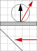
2. Perfect Mirrors

Shiny surface with complete specular reflection.
Reflection laws: L, N, R in same plane; incident angle = reflection angle (against normal),
but R is on the other side of the normal vector.

The result is, that we see a bright reflection spot where the camera lies in the R direction;
everywhere else the surface is dark !

3. Phong Approximation of Real Surfaces

Real surfaces are a mixture of chalky properties and of a dull, dusty mirror.
==> They have some diffuse as well as some specular reflection.
The reflected beam is spread out in a small angle around the unit vector R.
==> Phong model: Models the reflective component on a real surface as a "club" shape around R
Its intensity falls of with a user definable power of the cosine of the deviation angle from the ideal R direction.

Phong Illumination/Lighting/Surface Model:
Show effect of exponent of cosine function.

Phong Highlight on glossy surface:
Even uniform directional light falling on a flat surface can produce non-uniform brightntess,
if surface is partially reflective and we use a Phong illumination model.

4. Better Approximations of Real Surfaces:

Real materials are more complicated: Spreading of light (Phong exponent) may depend on:
   -- the incident angle {Torrence Sparrow model }.
   -- the color of the light {spectral behavior; different wavelenghts get absorbed/reflected differently.
   -- the surface material:
        -> in metal, reflected light penetrates deeper into substrate, picks up color of metal {metalness factor};
        -> on plastics, the light bounces off a surface layer, and keeps more of its own color composition.

Surface Characterization

Relationship between ka, kd, ks; and the C’s and the K’s

Shading Examples using spheres.

Brightness Normalization.

Normally one tries to carefully choose lights so that the produced brightnesses fall into the range 0 to 1.0,
which is then mapped onto the, say, 256 discrete beam intensities in the CRT.
In spite of best intentions the sum of all calculated brightnesses may exceed unity,
this may produce strange effects if left unchecked !
--> at the very least: clip to unity
--> better: detect this, and scale down all brightness values on object or in whole scene.

Now that we know what the brightness is that we would like to represent,
the question arises, how can we efficiently generate all the pixels of the right brightness ?

Shading and Rendering:

Techniques to produce desired display brightness -- efficiently !
We cannot afford to do a full shading calculation for each pixel.

Lambert lighting model + flat faces + uniform illumination -> easy:
==> ONE brightness value per polygon.
==> just take a representative value at centroid of face, and apply brightness values to all pixels of the polygon.
All other cases are harder: they result in non-uniform apparent brightness!

Causes of non-uniform brightness:

    -- Point light or spotlight close to surface.
    -- Curved surface where incident angle of light changes..
In both cases, one could sample more finely, and subdivide the surface patch into many smaller pieces.
    -- But this would still look patchy with sharp, contrasty brightness boundaries in between.
We need to smoothly blend these patches together!
    --> Sample illumination and calculate brightness at corners of patches
            and then interpolate between these sample points.
    -- We can cast this procedure into the framework of our scan-line algorithm,
        and do an interpolation similar to the interpolation of the z-values in the z-buffer.

1. Gouraud Shading Technique:
Linear interpolation of (scalar) brightness values

Good for: handling small nonuniformities in illumination intensity,
or for polyhedral approximations to round objects.
Principle: Use barycentric or bilinear (with sweep-line) intensity interpolation;
==> Implementation:
GOURAUD SHADING TECHNIQUE:

1. Compute shading at visual vertices, A, B, C, D ...
2. Compute shading along edges by linear interpolation between vertices.
3. Compute shading along spans by linear interpolation between edges.

Smooth shading can be applied whenever apparent brightness changes across a surface,
    -- either because the illumination is non-uniform,
    -- the reflection has highlights,
    -- or the surface is curved.

Faking smooth rounded objects:
Take an averaged brightness value at each corner,
derived from all incident lights and averaged vertex normals
(= vector sum of the face normals of all the adjacent polygons weighted by angle subtended at vertex).
The result is fake: edges remain straight (visible at the silhouette edges!) -- but it is efficient.

Limitations of Gouraud Shading:
Some flat spots; extrema may be "short-circuited"; discontinuities at concave corners; missing highlights...

2nd Technique: Phong Shading:
Interpolate normal vector directions

We can fix some of the above problems with a more sophisticated interpolation scheme.
PHONG SHADING

1. Compute normals at visual vertices, A, B, C, D ...
2. Compute normals along edges by vector interpolation.
3. Compute normals along spans by vector interpolation.
4.For every pixel compute brightness from interpolated normal direction and local light intensities.

Phong can interpolate over flat spots. -- But it is not perfect either !

Limitations of Phong Shading:
“Corrugated” structures with too few vertices (just a zig-zag)
may have all parallel normal directions and cannot represent periodic shading variations.
Geometry that is not seen at vertices cannot be inferred !
Illumination changes that are not seen at vertices cannot be inferred !

Reading Assignment:

Study: 2ndEd: Ch 6.1-6.5; Skim: 2ndEd: Ch 6.6-6.11.
Study: 3rdEd: Ch 6.1-6.5; Skim: 3ndEd: Ch 6.6-6.11.

New Homework Assignment:

ASG#8: "Lighting Calculations and Gouraud Shading "
This assignment can also be done with ANY PARTNER
-- possibly the one with whom you might do the final project.