ESPIRiT Reconstruction Demo

This is a demo on how to generate ESPIRiT maps and use them to perform ESPIRiT reconstruction for parallel imaging. It is based on the paper Uecker et. al, MRM 2013 DOI 10.1002/mrm.24751. ESPIRiT is a method that finds the subspace of multi-coil data from a calibration region in k-space using a series of eigen-value decompositions in k-space and image space. Here we also use the "soft" sense idea (Uecker et. al, "ESPIRiT Reconstruction using Soft-SENSE", Proceedings of the ISMRM 2013, pp-127) by using the eigen values to weight the eigen-vectors.

Contents

Prepare DATA

Here we perform ESPIRiT calibration on data which has strong aliasing in the phase-encode direction. SENSE often fails with this type of data.

load brain_alias_8ch
DATA = DATA/max(max(max(abs(ifft2c(DATA))))) + eps;
%DATA = crop(DATA,[256,256,8]);


ncalib = 24; % use 24 calibration lines to compute compression
ksize = [6,6]; % ESPIRiT kernel-window-size
eigThresh_k = 0.02 % threshold of eigenvectors in k-space
eigThresh_im = 0.9; % threshold of eigenvectors in image space
[sx,sy,Nc] = size(DATA);

% create a sampling mask to simulate x2 undersampling with autocalibration
% lines
mask = zpad(ones(sx,ncalib),[sx,sy]);
mask = repmat(mask,[1,1,8]);
mask(:,1:2:end,:) = 1;


DATAc = DATA.*mask;
calib = crop(DATAc,[sx,ncalib,Nc]);

eigThresh_k =

    0.0200

Display coil images:

im = ifft2c(DATAc);


figure, imshow3(abs(im),[],[1,Nc]);
title('magnitude of physical coil images');
colormap((gray(256))); colorbar;

figure, imshow3(angle(im),[],[1,Nc]);
title('phase of physical coil images');
colormap('default'); colorbar;

Compute Eigen-Value Maps

Maps are computed in two steps.

% compute Calibration matrix, perform 1st SVD and convert singular vectors
% into k-space kernels

[k,S] = dat2Kernel(calib,ksize);

idx = max(find(S >= S(1)*eigThresh_k));

Display the singular vectors and values of the calibration matrix

kdisp = reshape(k,[ksize(1)*ksize(2)*Nc,ksize(1)*ksize(2)*Nc]);
figure, subplot(211), plot([1:ksize(1)*ksize(2)*Nc],S,'LineWidth',2);
hold on,
plot([1:ksize(1)*ksize(2)*Nc],S(1)*eigThresh_1,'r-','LineWidth',2);
plot([idx,idx],[0,S(1)],'g--','LineWidth',2)
legend('signular vector value','threshold')
title('Singular Vectors')
subplot(212), imagesc(abs(kdisp)), colormap(gray(256));
xlabel('Singular value #');
title('Singular vectors')

crop kernels and compute eigen-value decomposition in image space to get maps

[M,W] = kernelEig(k(:,:,:,1:idx),[sx,sy]);

show eigen-values and eigen-vectors. The last set of eigen-vectors corresponding to eigen-values 1 look like sensitivity maps

figure, imshow3(abs(W),[],[1,Nc]);
title('Eigen Values in Image space');
colormap((gray(256))); colorbar;

figure, imshow3(abs(M),[],[Nc,Nc]);
title('Magnitude of Eigen Vectors');
colormap(gray(256)); colorbar;

figure, imshow3(angle(M),[],[Nc,Nc]);
title('Magnitude of Eigen Vectors');
colormap(jet(256)); colorbar;

Warning: Image is too big to fit on screen; displaying at 33% 
Warning: Image is too big to fit on screen; displaying at 33% 

Compute Soft-SENSE ESPIRiT Maps

crop sensitivity maps according to eigenvalues==1. Note that we have to use 2 sets of maps. Here we weight the 2 maps with the eigen-values

maps = M(:,:,:,end-1:end);

% Weight the eigenvectors with soft-senses eigen-values
weights = W(:,:,end-1:end) ;
weights = (weights - eigThresh_im)./(1-eigThresh_im).* (W(:,:,end-1:end) > eigThresh_im);
weights = -cos(pi*weights)/2 + 1/2;

% create and ESPIRiT operator
ESP = ESPIRiT(maps,weights);
nIterCG = 12;

Reconsturctions

ESPIRiT CG reconstruction with soft-sense and 2 sets of maps

disp('Performing ESPIRiT reconstruction from 2 maps')
tic; [reskESPIRiT, resESPIRiT] = cgESPIRiT(DATAc,ESP, nIterCG, 0.01,DATAc*0); toc

% ESPIRiT CG reconstruction with 1 map
disp('Performing SENSE reconstruction from 1 set of maps')
SNS = ESPIRiT(maps(:,:,:,end));
tic;[reskSENSE, resSENSE] = cgESPIRiT(DATAc, SNS, nIterCG,0.01 ,DATAc*0);toc

% GRAPPA reconstruction
disp('Performing GRAPPA reconstruction ')
tic; reskGRAPPA = GRAPPA(DATAc,calib,[5,5],0.01);toc
resGRAPPA = ifft2c(reskGRAPPA);

Performing ESPIRiT reconstruction from 2 maps
Elapsed time is 5.465768 seconds.
Performing SENSE reconstruction from 1 set of maps
Elapsed time is 4.023993 seconds.
Performing GRAPPA reconstruction 
reconstructing coil 1
reconstructing coil 2
reconstructing coil 3
reconstructing coil 4
reconstructing coil 5
reconstructing coil 6
reconstructing coil 7
reconstructing coil 8
Elapsed time is 12.164346 seconds.

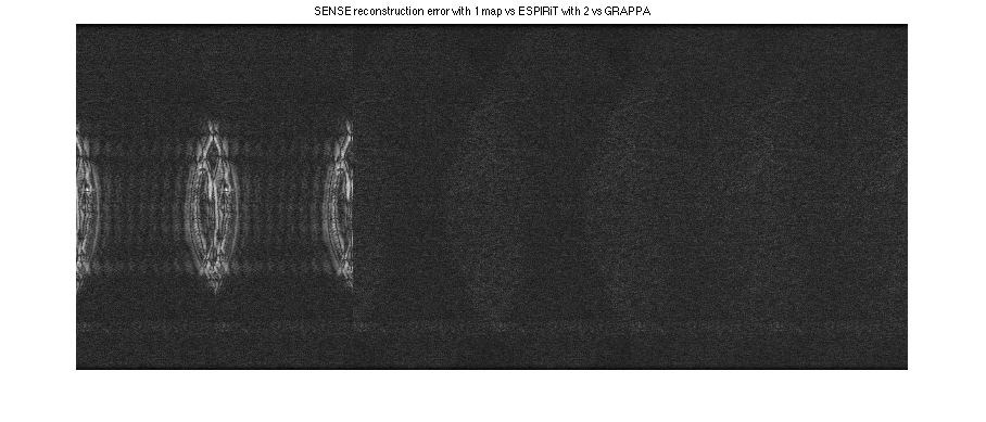
Note the typical center FOV aliasing in SENSE. Also, note that ESPIRiT has (very slightly) less error than GRAPPA

figure, imshow(cat(2,abs(resSENSE),sos(resESPIRiT), sos(resGRAPPA)),[])
title('SENSE reconstruction with 1 map vs ESPIRiT with 2 vs GRAPPA')
figure, imshow(cat(2,sos(ifft2c(reskSENSE-DATA)),sos(ifft2c(reskESPIRiT-DATA)),sos(ifft2c(reskGRAPPA-DATA))).^(1/2),[])
title('SENSE reconstruction error with 1 map vs ESPIRiT with 2 vs GRAPPA')

Published with MATLAB® R2013a