ESPIRiT Reconstruction with L1-Wavelet Demo
This is a demo on how to generate ESPIRiT maps and use them to perform ESPIRiT reconstruction for parallel imaging. It is based on the paper Uecker et. al, MRM 2013 DOI 10.1002/mrm.24751. ESPIRiT is a method that finds the subspace of multi-coil data from a calibration region in k-space using a series of eigen-value decompositions in k-space and image space. Here we also use the "soft" sense idea (Uecker et. al, "ESPIRiT Reconstruction using Soft-SENSE", Proceedings of the ISMRM 2013, pp-127) by using the eigen values to weight the eigen-vectors.
Contents
Prepare DATA
Here we perform ESPIRiT calibration on data which has strong aliasing in the phase-encode direction. SENSE often fails with this type of data.
load brain_8ch
DATA = DATA/max(max(max(abs(ifft2c(DATA))))) + eps;

ksize = [6,6]; % ESPIRiT kernel-window-size
eigThresh_k = 0.02; % threshold of eigenvectors in k-space
eigThresh_im = 0.9; % threshold of eigenvectors in image space

% parameters for L1-reconstruction with splitting
nIterCG = 5;       % number of CG iterations for the PI part
nIterSplit = 15;    % number of splitting iterations for CS part
splitWeight = 0.4;  % reasonable value
lambda = 0.0025;    % L1-Wavelet threshold


[sx,sy,Nc] = size(DATA);

% create a sampling mask to simulate x2 undersampling with autocalibration
% lines
mask = mask_randm_x4;
mask = repmat(mask,[1,1,8]);
ncalib = getCalibSize(mask_randm_x4);


DATAc = DATA.*mask;
calib = crop(DATAc,[ncalib,Nc]);
Display coil images:
im = ifft2c(DATAc);


figure, imshow3(abs(im),[],[1,Nc]);
title('magnitude of physical coil images');
colormap((gray(256))); colorbar;

figure, imshow3(angle(im),[],[1,Nc]);
title('phase of physical coil images');
colormap('default'); colorbar;


Compute Eigen-Value Maps
Maps are computed in two steps.
% compute Calibration matrix, perform 1st SVD and convert singular vectors
% into k-space kernels

[k,S] = dat2Kernel(calib,ksize);

idx = max(find(S >= S(1)*eigThresh_k));
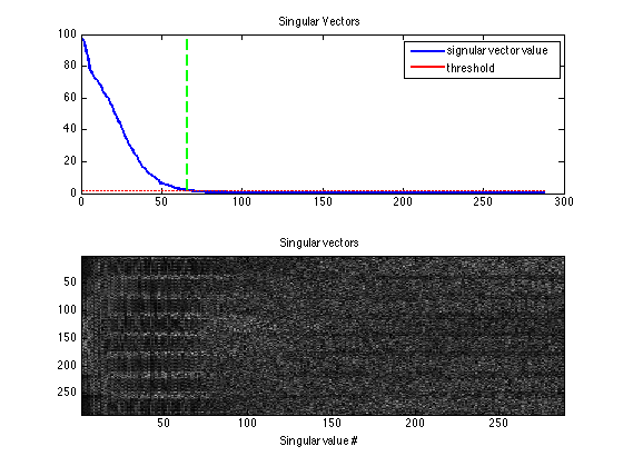
Display the singular vectors and values of the calibration matrix
kdisp = reshape(k,[ksize(1)*ksize(2)*Nc,ksize(1)*ksize(2)*Nc]);
figure, subplot(211), plot([1:ksize(1)*ksize(2)*Nc],S,'LineWidth',2);
hold on,
plot([1:ksize(1)*ksize(2)*Nc],S(1)*eigThresh_k,'r-','LineWidth',2);
plot([idx,idx],[0,S(1)],'g--','LineWidth',2)
legend('signular vector value','threshold')
title('Singular Vectors')
subplot(212), imagesc(abs(kdisp)), colormap(gray(256));
xlabel('Singular value #');
title('Singular vectors')
crop kernels and compute eigen-value decomposition in image space to get maps
[M,W] = kernelEig(k(:,:,:,1:idx),[sx,sy]);
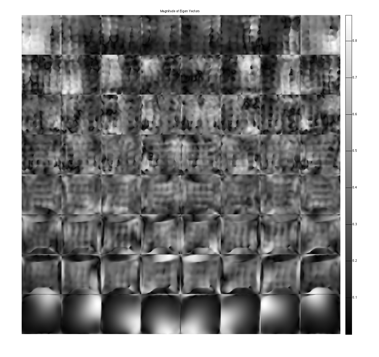
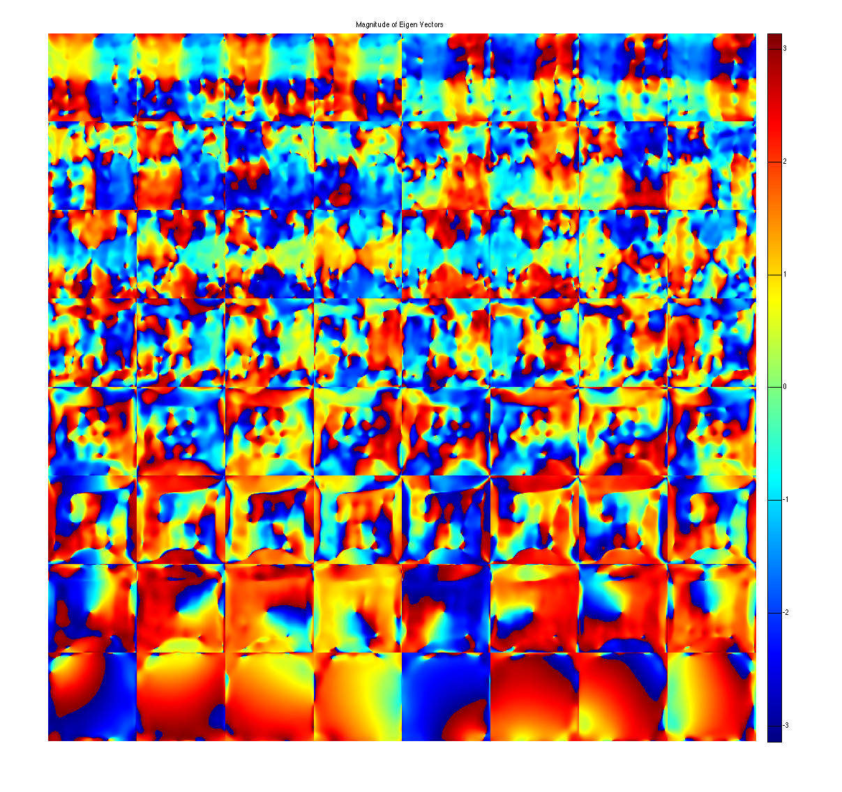
show eigen-values and eigen-vectors. The last set of eigen-vectors corresponding to eigen-values 1 look like sensitivity maps
figure, imshow3(abs(W),[],[1,Nc]);
title('Eigen Values in Image space');
colormap((gray(256))); colorbar;

figure, imshow3(abs(M),[],[Nc,Nc]);
title('Magnitude of Eigen Vectors');
colormap(gray(256)); colorbar;

figure, imshow3(angle(M),[],[Nc,Nc]);
title('Magnitude of Eigen Vectors');
colormap(jet(256)); colorbar;
Warning: Image is too big to fit on screen; displaying at 67%
Warning: Image is too big to fit on screen; displaying at 67%

Compute Soft-SENSE ESPIRiT Maps
crop sensitivity maps according to eigenvalues==1. Note that we have to use 2 sets of maps. Here we weight the 2 maps with the eigen-values
maps = M(:,:,:,end-1:end);

% Weight the eigenvectors with soft-senses eigen-values
weights = W(:,:,end-1:end) ;
weights = (weights - eigThresh_im)./(1-eigThresh_im).* (W(:,:,end-1:end) > eigThresh_im);
weights = -cos(pi*weights)/2 + 1/2;

% create and ESPIRiT operator
ESP = ESPIRiT(maps,weights);
Reconsturctions
ESPIRiT CG reconstruction with soft-sense and 1 sets of maps
XOP = Wavelet('Daubechies_TI',4,6);
FT = p2DFT(mask,[sx,sy,Nc]);

disp('Performing ESPIRiT reconstruction from 2 maps')
tic; [reskESPIRiT, resESPIRiT] = cgESPIRiT(DATAc,ESP, nIterCG*3, 0.01,DATAc*0); toc

disp('Performing L1-ESPIRiT reconstruction from 2 maps')
tic
[resL1ESPIRiT] = cgL1ESPIRiT(DATAc, resESPIRiT*0, FT, ESP, nIterCG,XOP,lambda,splitWeight,nIterSplit);
toc

% GRAPPA reconstruction
disp('Performing GRAPPA reconstruction ... slow in Matlab! ')
tic; reskGRAPPA = GRAPPA(DATAc,calib,[5,5],0.01);toc
resGRAPPA = ifft2c(reskGRAPPA);
Performing ESPIRiT reconstruction from 2 maps
Elapsed time is 3.460917 seconds.
Performing L1-ESPIRiT reconstruction from 2 maps
Iteration: 1, consistency: 18.537199
Iteration: 2, consistency: 6.907292
Iteration: 3, consistency: 4.212248
Iteration: 4, consistency: 3.600387
Iteration: 5, consistency: 3.386763
Iteration: 6, consistency: 3.279046
Iteration: 7, consistency: 3.215016
Iteration: 8, consistency: 3.173626
Iteration: 9, consistency: 3.145386
Iteration: 10, consistency: 3.125352
Iteration: 11, consistency: 3.110704
Iteration: 12, consistency: 3.099735
Iteration: 13, consistency: 3.091360
Iteration: 14, consistency: 3.084862
Iteration: 15, consistency: 3.079751
Elapsed time is 22.371217 seconds.
Performing GRAPPA reconstruction ... slow in Matlab!
reconstructing coil 1
reconstructing coil 2
reconstructing coil 3
reconstructing coil 4
reconstructing coil 5
reconstructing coil 6
reconstructing coil 7
reconstructing coil 8
Elapsed time is 225.601446 seconds.
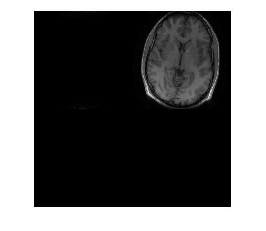
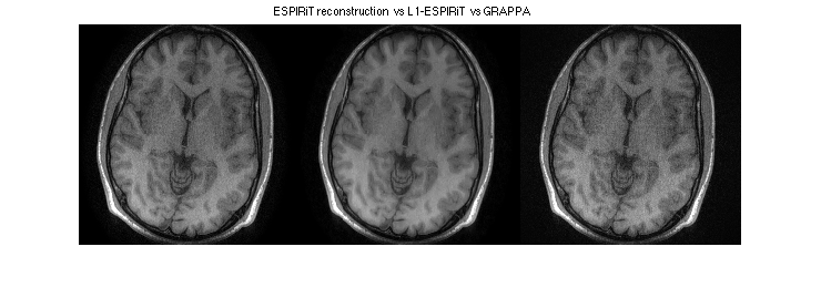
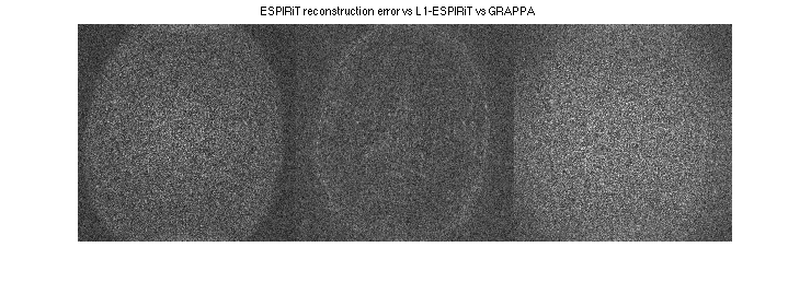
Note the typical center FOV aliasing in SENSE. Also, note that ESPIRiT has (very slightly) less error than GRAPPA
figure, imshow(cat(2,sos(resESPIRiT), sos(resL1ESPIRiT),sos(resGRAPPA)),[0,1]);
title('ESPIRiT reconstruction  vs L1-ESPIRiT  vs GRAPPA')
figure, imshow(cat(2,sos(ifft2c(reskESPIRiT-DATA)),sos(ifft2c(fft2c(ESP*resL1ESPIRiT)-DATA)),sos(ifft2c(reskGRAPPA-DATA))).^(1/2),[])
title('ESPIRiT reconstruction error vs L1-ESPIRiT vs GRAPPA')
