Geometric Decomposition Coil Compression

This is a demo of the ESPIRiT Coil Compression (ECC). It is based on the abstract: D. Bahri et. al, "ESPIRiT-Based Coil Compression for Cartesian Sampling" ISMRM 2013 pp:2657

The demo shows how to use the compression and in addition it shows the use of alignment of the compression matrices. The example is on 2D data, but can also be applied on 3D as well. ECC removes correlations between channels along a fully sampled readout dimension. This allows for significant reduction in data, so parallel imaging and other multi-channel algorithms are much more computationally efficient. This demo demonstrate effective compression from 32->5 virtual channels. ECC has better noise properties than GCC.

Contents

Set parameters:

load brain_32ch.mat

% number of compressed virtual coils
ncc = 5;
dim = 2;
ncalib = 24; % use 24 calibration lines to compute compression
[sx,sy,Nc] = size(DATA);

slwin = 4; % sliding window length for GCC

dispm = [4,8]; % diplay matrix settings

% crop calibration data
calib = crop(DATA,[ncalib,sy,Nc]);

ECC - ESPIRiT Coil Compression (with no alignment)

This code computes ECC compression matrices from calibration data. The data is the transformed to the new compressed virtual coils basis.

eccmtx = calcECCMtx(calib,dim,ncc);

% compress the data
ECCDATA = CC(DATA,eccmtx,dim);

% compute coil image
ECCim = ifft2c(ECCDATA);

% Also compute GCC for comparison
gccmtx = calcGCCMtx(calib,dim,slwin);
% compress the data
GCCDATA = CC(DATA,gccmtx,dim);
% compute coil image
GCCim = ifft2c(GCCDATA);

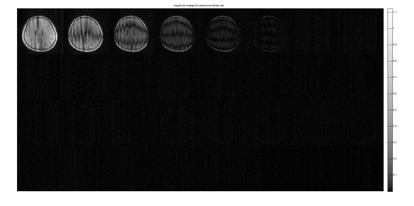
The compressed virtual coil domain shows that the data can be represented effectively by 5 out of 32 channels. The error is much lower than in SCC.

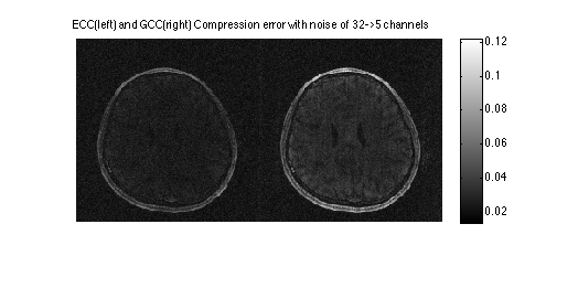
Note that the ECC error image is noisier than the GCC. This is because more noise is left out of image, whereas GCC is biased and fits some noise.

Note that the colormap is non-linear to improve dynamic-range of the visualization.

figure, imshow3(abs(ECCim),[],dispm);
title('magnitude unaligned compressed virtual coils');
colormap(sqrt(gray(256))); colorbar;

figure, imshow3(angle(ECCim),[],dispm);
title('phase unaligned compressed virtual coils');
colormap('default');
colorbar

figure, imshow(cat(2,sos(ECCim(:,:,ncc+1:end)),sos(GCCim(:,:,ncc+1:end))),[]);
colorbar;
title('ECC(left) and GCC(right) Compression error of 32->5 channels')

ESPIRiT Coil Compression (with alignment)

Here, we crop the compression matrices so they compress from 32->5 channels. We then align the matrices so they smoothly vary. This does not change the subpspace of the data -- only rotates the basis vectors.

Note that the colormap is non-linear to improve dynamic-range of the visualization.

% crop and align matrices
eccmtx_aligned = alignCCMtx(eccmtx(:,1:ncc,:));

% compress the data
ECCDATA_aligned = CC(DATA,eccmtx_aligned, dim);

% compute coil image
ECCim_aligned = ifft2c(ECCDATA_aligned);

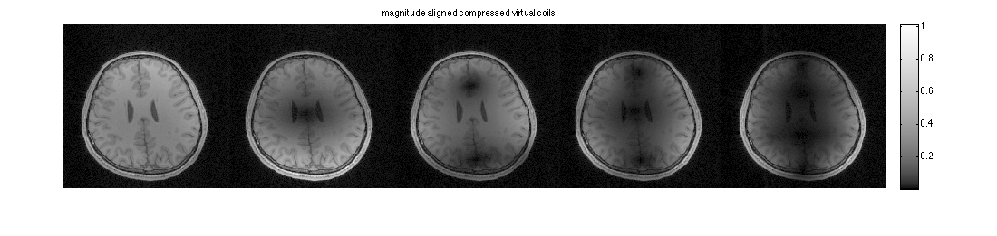
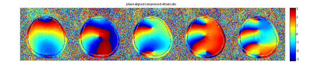
The compressed virtual coil are now smooth in phase and magnitude

figure, imshow3(abs(ECCim_aligned),[],[1,ncc]);
title('magnitude aligned compressed virtual coils');
colormap(sqrt(gray(256))); colorbar;

figure, imshow3(angle(ECCim_aligned),[],[1,ncc]);
title('phase aligned compressed virtual coils');
colormap('default');
colorbar

ECC - ESPIRiT Coil Compression with added noise

Here we add noise to the calibration data -- compute ECC and GCC compression matrices and then use them to compress the original data.

ECCerr = zeros(15,1);
GCCerr = zeros(15,1);
sigma = logspace(log10(0.001),log10(0.05),15);

% repear compression for increased noise levels and comput squared error
for n=1:15

    calib_n = calib + randn(size(calib))*sigma(n)/sqrt(2) + 1i*randn(size(calib))*sigma(n)/sqrt(2);
    eccmtx = calcECCMtx(calib_n,dim,ncc,6);
    % compress the data
    ECCDATA = CC(DATA,eccmtx,dim);
    % compute coil image
    ECCim = ifft2c(ECCDATA);

    % Also compute GCC for comparison
    gccmtx = calcGCCMtx(calib_n,dim,slwin);
    % compress the data
    GCCDATA = CC(DATA,gccmtx,dim);
    % compute coil image
    GCCim = ifft2c(GCCDATA);

    ECCerr(n) = sum(sum(sos(ECCim(:,:,ncc+1:end)).^2));
    GCCerr(n) = sum(sum(sos(GCCim(:,:,ncc+1:end)).^2));
end

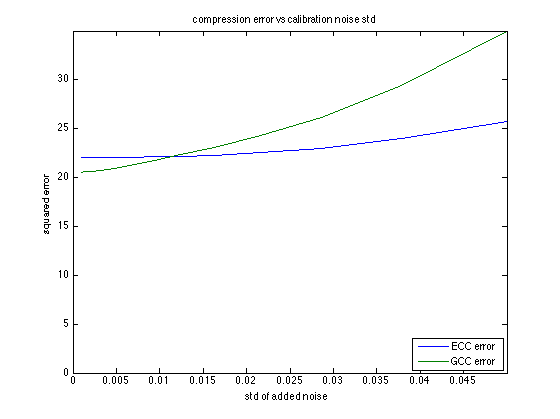
GCC has slightly lower error for low level of noise. However, ECC has quite stable performance with increasing noise, whereas GCC is degrading rapidly.

figure, plot(sigma,ECCerr,sigma,GCCerr)
title('compression error vs calibration noise std')
xlabel('std of added noise')
ylabel('squared error');
axis([0,sigma(end),0,max(GCCerr(end),ECCerr(end))])
legend('ECC error', 'GCC error','Location','SouthEast');

figure, imshow(cat(2,sos(ECCim(:,:,ncc+1:end)),sos(GCCim(:,:,ncc+1:end))),[]);
colorbar;
title('ECC(left) and GCC(right) Compression error with noise of 32->5 channels')

Published with MATLAB® R2013a