Designed by Professor C. J. Spanos, implemented by Yuri Yuryev
In every wireless communication system the actual transmission of the waves over the air is carried out by some sort of an antenna system. An important aspect of an antenna is its radiation pattern. Radiation patterns are affected by such factors as mounting height, position angle, soil conductivity, foreign conductors, air humidity, etc.
However, scattering matrix analysis is a useful tool for the examination of the radiation pattern of any system at its individual site. The calculation of the S-parameters is done with a Network Analyzer, which we will use for this experiment. Please review the S-parameter theory including the 2-port model before participating in this lab.
The two ports of the system in our experiment are made of the car-phone antenna
(technically an 860 MHz center-loaded vertical 5/8 ![]() antenna with a ground plane), and a
receiving antenna, consisting of a magnetic coil. ``Center-loaded'' refers to the coil in the
mid-section of the antenna. The role of this coil is to make this antenna look like a 50 ohm
load at the resonant frequency. Without it the antenna will have a strong capacitive impedance
component, and it will not match the transmission line for best power transfer. It is important
to remember that to the signal traveling in the transmission line, the antenna looks like an
impedance load
R+jX, perhaps complex, but ideally just 50 ohms.
antenna with a ground plane), and a
receiving antenna, consisting of a magnetic coil. ``Center-loaded'' refers to the coil in the
mid-section of the antenna. The role of this coil is to make this antenna look like a 50 ohm
load at the resonant frequency. Without it the antenna will have a strong capacitive impedance
component, and it will not match the transmission line for best power transfer. It is important
to remember that to the signal traveling in the transmission line, the antenna looks like an
impedance load
R+jX, perhaps complex, but ideally just 50 ohms.
The system that we will use functions in the following way: signals of different frequencies will be sent by the Network Analyzer between the transmitting vertical antenna, and the receiving coil. Assuming that the two antennae are far enough apart to ignore near fields, between the two antennae, the signals travel by means of EM radiation. By analyzing the scattering matrix of this system we will try to find the basic radiation patterns of a simple vertical antenna.
Vertical antennae have a cylindrically symmetric (omni-directional) radiation pattern, which is very useful in situations when you want to transmit and receive the same no matter which direction you are facing. When driving, for example, many of us use a vertical antenna for receiving broadcast FM stations, and the reception is more or less the same no matter which way our car is facing.
However, for other operations we need antennae with directional gain. This means that some antennae have a front and a back. A typical application for a ``gain'' antenna is for receiving TV broadcasts. Directivity here helps zero in on the signal, while attenuating signal reflections that might a arrive a bit later from other directions and show up on the TV screen as ``ghosts''. Another reason for directional antennae is that, in their optimum direction, they will receive a stronger signal than a comparable omni-directional antenna.
For many applications the choice of the best directional gain antenna usually falls on Yagi-Uda arrays. Yagi arrays usually consist of a radiating dipole, reflector elements and director elements. The distance between the elements is such that through coupling, currents are induced into the elements by the dipole phased in a way as to create a radiation/receiving pattern that favors one direction. We will examine such a system in the second part of the lab.
Note that in this experiment your measurements will be very approximate, because of stray reflections from the objects surrounding your antennae.
The purpose of this demonstration is to use the concept of the scattering matrix in order
to measure the transmission between two ports consisting of a 5/8 ![]() , loaded, ground plane
cell phone ``transmitting'' antenna and a small ``receiving'' magnetic loop. By measuring the
two-port scattering matrix elements S11, S12, S21 and S22 using a Network Analyzer one can
determine the kind of load the antenna presents to the transmitter over a range of frequencies,
the kind of load the loop presents to the transmitter, and the type of signal attenuation between
the antenna and the receiving loop. If one plots S21 (or S12, since this is a ``reciprocal''
network) as a function of the position of the loop, one can then plot the radiation pattern of
the antenna.
, loaded, ground plane
cell phone ``transmitting'' antenna and a small ``receiving'' magnetic loop. By measuring the
two-port scattering matrix elements S11, S12, S21 and S22 using a Network Analyzer one can
determine the kind of load the antenna presents to the transmitter over a range of frequencies,
the kind of load the loop presents to the transmitter, and the type of signal attenuation between
the antenna and the receiving loop. If one plots S21 (or S12, since this is a ``reciprocal''
network) as a function of the position of the loop, one can then plot the radiation pattern of
the antenna.
Power up the HP Network Analyzer. Press the Cal Button. Choose ``Calibrate Menu", ``full 2-port", and then ``Reflection" from soft keys menu. Remove everything from the ports so that the brass connectors are showing. Choose ``S11 Open" and ``S22 Open" from the soft key menu. Acquire a short terminator from the HP Calibration Kit, attach it to port 1 and press ``S11 Short". Repeat with the short for port 2. Place a 50 ohm load on port 1 and press ``Load". Repeat with the load for port 2. Now we are finished with the reflection part of the calibration--press ``Reflection Done". Choose ``Transmission'' from the soft keys. Short port 1 to port 2 using the coax from the receiving magnetic loop. To calibrate press all soft keys starting from the top in the sequence 1, 2, 4, 3, so that the final line on the display is a horizontal. Choose ``Transmission Done" Now select ``Isolation", then press ``Omit Isolation", ``Done" and ``Done 2-port" soft keys in the above sequence. Then press ``SaveReg 1". You are now finished with the calibration.
Attach the antenna coax to port 1 and the receiving loop coax to port 2. Select the frequency span
to be 800-905 MHz. From the format menu select the SWR display for S11 and find the resonant
frequency and standing wave ratio of the antenna:
Resonant Frequency MHz; SWR .
Now switch to dual display by pressing ``Display", ``On". Select Ch. 2--now you are
operating on the bottom display. Press ``Meas" button and choose ``Trans: FWD S21, [B/R]".
Select the format of the bottom display to be logarithmic, and auto-scale the display from the
``Scale Ref" menu.
What does the bottom window display?
How would it change if you selected S12, from the menu? Explain.
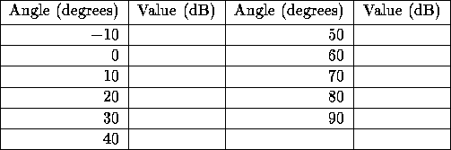
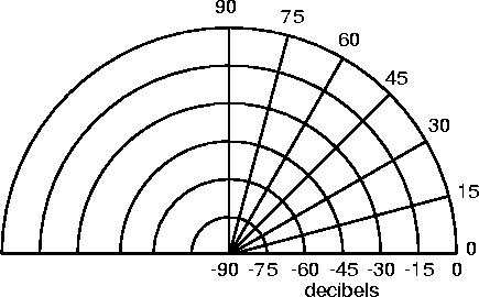
Slip the receiving coil through a loop in the string attached to the base of the antenna. Measure
the strength of signal in dB in the range of (-10, 90) degrees to the ground plane in 10 degree
increments. Keep the plane of the receiving loop perpendicular to the floor at all times--this
will restrict your measurement to the component of the magnetic field vector in the azimuthal
( ![]() ) direction. Plot the measured signal strength on the graph provided below.
) direction. Plot the measured signal strength on the graph provided below.
Table 1: Measured S21 Pattern
Attach the 3-element Yagi antenna to the output of the signal generator. Enter the frequency of 146.00 MHz and amplitude of +0.0 dBm, with zero modulation. Attach the RF probe to the HP Spectrum Analyzer. Set the frequency scan from 140 MHz to 150 MHz. Set the sweep time to 300 ms. You should see a spike at 146 MHz on the display. Position the marker on top of the spike. In the top right hand corner you should see the signal strength of the antenna in dBm (decibels referenced to 1 milliwatt).
Rotate the antenna and mark the position that shows the strongest signal. The antenna
front-to-back ratio is the difference between its best gain and the gain 180 degrees away from its
best gain. Measure the antenna front-to-back ratio.
Front-to-back ratio = max signal (dB) - signal at ![]() off (dB) = .
off (dB) = .
Measure the antenna gain in dBd (referenced to a dipole) by removing the reflector (the longer
of the three elements) and the director (the shorter of the three elements) and noting the signal
strength of the remaining dipole:
Gain = dBd.
Note that the dipole after the director and reflector are removed is not resonant, i.e., it does
not present the transmission line with a 50 ohm termination any more. Use the Network Analyzer
to measure the SWR of the Yagi antenna at 146 MHz with and without the reflector and director
elements. Record the two values below:
SWR of complete antenna = .
SRW of antenna without reflector and director elements = .
Because the antenna is no longer matched, the coaxial cable losses are about
1 dB greater than when the load was matched. Use this information to ``correct'' your estimate of
the antenna gain.
Corrected antenna gain estimate = dBd.