Spectral Filters in the Bullfrog Ear

Notes from seminar given August 13, 2008, Univ. of Oregon

1. Why Spectral Filters?

What are their selective advantages?

a. Rejection of noise and interference

Example:

• Presume that the bullfrog sacculus is a micro-seismic sensor whose function (adaptive value) lies in its ability to alert the frog to significant vibrations in the ground—such as the footfalls of predators.

• The amplitude of micro-seismic noise on the earth’s surface is very high at frequencies below about 5 Hz.

• Signals from footfalls and other impulsive micro-seismic stimuli in the ground have spectral peaks at higher frequencies (usually centered about 50 Hz).

• To detect these, it would be appropriate to suppress saccular inputs in the in the frequency range below 5 Hz.

• Responses to those inputs could mask or interfere with responses to the vibrations from predator footfalls.

• Being supersensitive to vibration, the bullfrog sacculus is sensitive to airborne sound as well— responses to which also could mask or interfere with the signals in the ground.

• The bullfrog amphibian papilla responds to the acoustic spectrum for several octaves, beginning at about 100 Hz.

• Therefore it would be appropriate to suppress saccular inputs in the frequency range above approx. 100Hz..

• By focusing on the spectral region between about 5 Hz and about 100 Hz, the bullfrog sacculus would cover most of the spectral energy of footfalls, while suppressing interference from a wide range of other sources.

b. Spectro-temporal analysis

Example

• Separation of signals from one another is a quintessential part of hearing.

• The acoustic input arriving at each ear commonly is a mixture of sounds from many sources. Each of the two cochleae carries out an ongoing spectrographic decomposition of its acoustic input, the human brain then is able to infer (computationally) which spectro-temporal components belong to a single waveform (from a single source) . . .

• and to recombine those components to form a perception of that waveform.*

• The computations require spectro-temporal decomposition with high resolution in both frequency and time.

• This can be achieved with filter functions (impulse responses) that are compact in time and still provide sharp spectral discrimination - - -

• implying the use of very steep band edges rather than very narrow pass-bands for spectral discrimination.

• By extension, I presume that non-human listeners employ comparable computations with the same filter requirements.

* Perception, of course, is a mental construction. Investigators depend on reporting from human subjects in order to infer that a particular perception has occurred. Understanding the linkage between neural constructions underlying perceptions and perceptions themselves still seems beyond the reach of natural science. The psychophysicist bridges that gap by mapping observable physical parameters (e.g., of complex acoustic waveforms) to reportable perceptions. The neural algorithms and filter requirements for spectral decomposition in the human listener have been inferred, strongly, from auditory psychophysics.

2. Examples of acoustic filters in the vertebrate ear

Here are filter functions from gerbil, turtle and bullfrog ears, observed at common background sound levels - - - 40 decibels and above

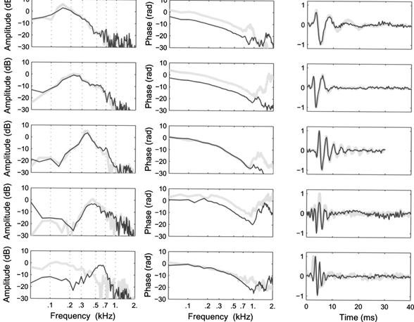
a. Sample filter functions (impulse responses) from gerbil cochlear units, with spectral peaks at approximately ½-octave intervals (Lewis, Henry, Yamada, 2002)

Note: the filter functions on the left were estimated by REVCOR (1^st-order Wiener kernels).

Those on the right were derived from decomposition of the 2^nd-order Wiener kernels (see

“Saccular physiology from the outside,” part I).

Amplitude DFTs (Discrete Fourier Transforms) of the same gerbil filter functions

The noisiness of these Discrete Fourier Transforms reflects the noisiness inherent in the

impulse-response estimation procedure (reverse correlation of spike occurrences with

broad-band noise stimuli). From the noisy base in each DFT rises the relatively

smooth tuning peak of the unit.

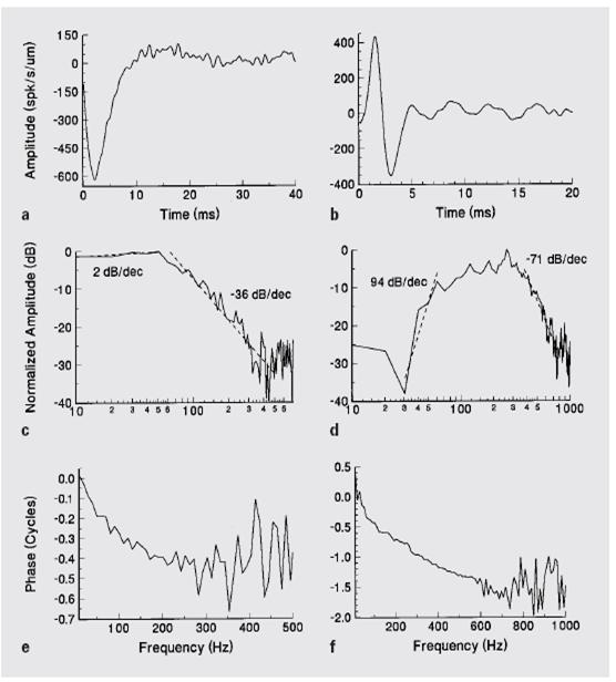
b. How faithfully do the filter functions represent the actual filters?

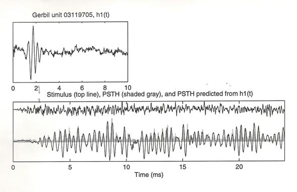
The upper frame shows the filter function, h₁(t). It was computed for a gerbil cochlear unit by reverse (triggered) correlation between continuous (non-repeating) noise stimulus and the unit’s spikes. In the lower frame, the top line shows a different broad-band noise waveform that was presented repeatedly—as a closed-field airborne sound stimulus to the gerbil’s ear canal. Beneath that, in gray, is the spike-rate response (Peri-Stimilus Time Histogram) of the same gerbil unit to this same, repeated stimulus. The superimposed solid line is the spike-rate response predicted from the filter function (the convolution of the filter function with the repeated waveform). The filter function clearly predicts the amplitudes and phases of the positive spike-rate peaks beautifully. It fails to reflect at all, however, the fact that spike rates cannot be negative. The strong clipping, imposed by that fact, can be eliminated experimentally by adding non-repeating dithering noise to the repeated stimulus waveform. Even without that, the results shown here strongly support the fidelity of the filter function in representing the tuning and timing of this gerbil unit’s response. Furthermore, the filter functions all are compact in time and yield tuning curves with steep band edges.

c. Sample filter functions from the basilar papilla of the red-eared turtle (Sneary & Lewis 2007)

The filter functions are displayed in the right-hand column, the amplitude and phase

components of their DFTs are displayed in the left- and center columns, respectively.

• In this ancient reptile, the filter functions are compact,

• but the band edges are not nearly as steep as they are in the gerbil.

• What about the American bullfrog, a relatively recent amphibian?

d. Sample filter-function DFTs from the American Bullfrog

These are Bode plots (log-log plots of DFTs) of filter functions taken

by Xiaolong Yu (XLY), Walter Yamada (WMY) and Kathy Cortopassi

(KAC). Representative filter functions themselves (impulse responses)

are shown below and in the section (“Saccular physiology from the outside,

part I” under Sacculus). Notice that, like the mammalian cochlea, the

amphibian papilla covers its frequency range with an array of filters, each

covering only part of the total range. As in the cochlea, these are

distributed tonotopically over the papillar surface-- high-frequency

sensitivity at one end, low-frequency at the other.

• Bullfrog band edges are very steep.

• How might they be they achieved?

• For the answer– we’ll do a little circuit analysis . .

We’ll consider models of discrete processes only - - - no distributed models of spatially-extensive wave or diffusion processes. In finite-element representations of diffusion or waves, the behaviors of the two kinds of models converge, so we lose no generality.

3. How Spectral Filters?

All classical physical processes can be described in terms of non-equilibrium thermodynamics, which in turn is describable in terms of a small set of generalized dynamic elements. In other words, with this small set of elements, one can faithfully model the dynamics of all such processes—including the processes that might underlie the peripheral filters of the vertebrate ear. A broad subset of such processes are faithfully represented by compartmental models (familiar to most biologists), where each compartment represents a site or state in which some entity can accumulate, and transfer between such sites or states is accomplished by first-order kinetics—as in linear chemical kinetics, diffusion across osmotic barriers, and heat flow. We shall begin by determining whether or not the observed filter properties could arise with such processes alone.

a. Compartmental models

Three-compartment model I

This represents a three-state process (e.g. chemical reaction or diffusion) with linear kinetics.

When J_in is an impulse at t = 0, all the internal variables have the form …..

A e^-0.20t + B e^-1.56t + C e^-3.25t

and the corner frequencies (rad/s) of the system are: 0.20 1.56 3.25

Three faces of A e^-0.20t + B e^-1.56t + C e^-3.25t

Although the functions Q₁(t), Q₂(t), and Q₃(t) have the same basic mathematical form,

they are distinctively different in shape—depending (mathematically) on the magnitudes

and signs of the parameters (A,B,C) and (physically) on the position of the compartment

relative to the input. The impulsive input fills the first compartment instantly (in our simple

model); the second compartment fills as the first gradually drains into it; and the third fills

even more gradually as the second compartment drains into it.

• Each compartment behaves as a leaky integrator

• At frequencies well below the lowest corner (0.20 rad/s), the system is always very close to steady state (leaks dominate):

• If Jin = K mol per s

• then Q1 = 3K mol

• Q2 = 2K mol

• and Q3 = K mol

• At frequencies well above the highest corner (3.25 rad/s), the compartments don’t have time to leak significantly during each half cycle,

• They approximate pure integrators,

• and the system approximates closely its asymptotic behavior …..

The half-cycle volume (integral) of sinusoidal flow
decreases as the reciprocal of frequency

Notice that, for a sine wave of constant amplitude, the area under each half cycle

decreases in inverse proportion to the frequency. In our model, positive areas

(areas above the baseline) represent accumulation (of whatever is reacting or diffusing)

in a compartment. Negative areas (below the baseline) represent depletion. Over

a full sinusoidal cycle the amount accumulation equals the amount of depletion. The

amount of accumulated stuff is maximum each time the positive half-cycle is complete.

Asymptotic responses at high frequencies

Bode plots (DFTs) of the three faces of
A e^-0.20t + B e^-1.56t + C e^-3.25t

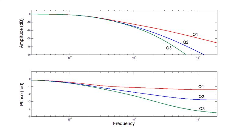
The corners separating the very-low frequency behavior (response amplitudes of all quantities

remain constant) and the very-high frequency behavior (response amplitudes decline at slopes

that are constant on the log-log plot) are very rounded, extending over a decade of frequency.

They are not nearly as sharp or abrupt as those we see in the data for any of the four inner-ear

organs discussed here.

· We can, however, make the following, very general statements about our observations of filter properties in the ear . . . . .

Rules of thumb

• The Bode (DFT) plot should provide strong inference regarding the number (N) of separate integrating processes, in cascade, between the point of observation and the point of input.

• The magnitudes of the asymptotic slopes should sum to N, corresponding to 1/w^N

• This is the same as 6N dB per octave and 20N dB per decade

• The range of phase change should be Np/2 radians (90N degrees)

Now we can attempt to sharpen the corners in our amplitude Bode plots.

Three-compartment model II

corner frequencies (rad/s): 1.00 1.00 1.00

With its unidirectional coupling from state to state, this three-compartment model is unrealizable, in principle, with passive nonequilibrium thermodynamic processes. Nevertheless, it can be approached as closely as one might wish with standard chemical or diffusional kinetics. Its impulse response will reflect n identical corner frequencies when its response is observed at the nth compartment in the sequence. If it were extended to six compartments (see below), the last one in the sequence would exhibit six identical corner frequencies of 1.0 rad/s.

Among all n-compartment models, the one with n identical corner frequencies has the sharpest corner in its amplitude Bode diagram (the graph of the amplitude part of its discrete Fourier transform or DFT). It’s the best we can do with cascades of first-order kinetics.

Here are impulse responses for the nth compartment, with n being one, two and six.

Here are Bode plots for the same three impulse responses (graphs of the amplitude

and phase parts of their DFTs). These all are low-pass filters.

Toward the end of this presentation we’ll see low-pass filter functions from the bullfrog lagena. Other filter functions from the lagena are band-pass in nature, as are all of the filter functions we have observed from the bullfrog sacculus, AP and BP.

• To create a band-pass filter, we must add differentiation—

• (in cascade (series), anywhere along the cascade of leaky integrators).

Impulse responses of Model II with six leaky integrators

and 0, 1, 2 & 3 stages of differentiation

The impulse responses are plotted in the top frame, the amplitude parts of their DFTs are plotted in the lower frame. In the top frame, the inserted numbers indicate the number of stages of differentiation for each plot. In the lower frame, the numbers on the left indicate both the number of differentiation stages and the asymptotic slope at low frequency. The numbers on the right indicate the asymptotic slopes at high frequency.

Our rules of thumb are augmented by one additional statement:

• The slope of the low-frequency asymptote equals the number of stages of differentiation.

The rest remain valid . . .

• The magnitudes of the asymptotic slopes of the amplitude Bode plots still sum to N (the number of separate integrating processes in cascade between the point of stimulus input and the point of observation).

• The phase range remains Np/2 rad.

Based on identical corner frequencies, the amplitude DFT plots (Bode plots) shown here illustrate the sharpest filters available with N (six in this case) first-order kinetic processes. Now we can compare this best-case result with filter functions from the bullfrog ear.

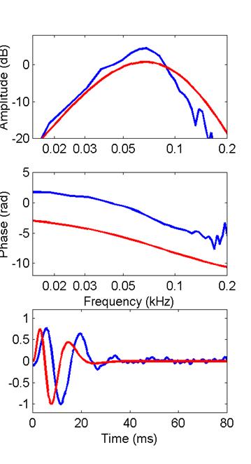
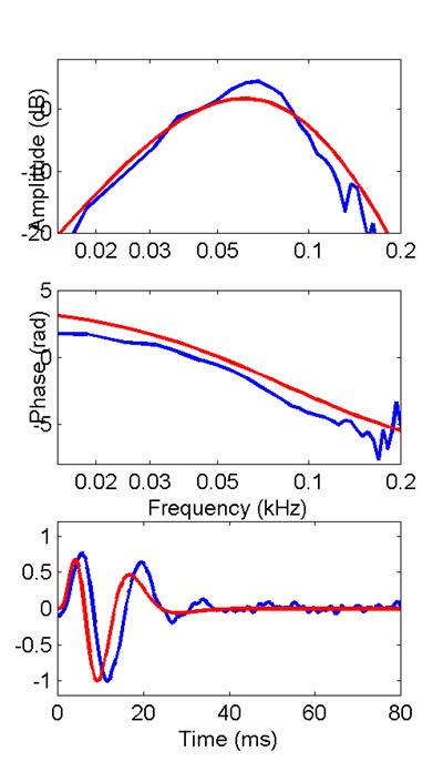
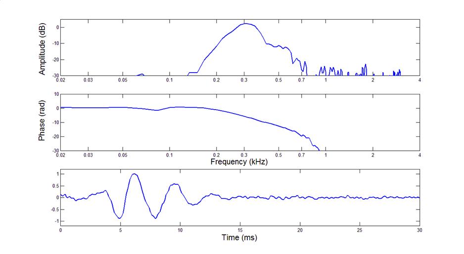
Here is the filter function from a saccular unit (recorded by Xiaolong Yu). The impulse response is plotted in the bottom frame; its Bode plots are above it. The low- and high-frequency slopes of the amplitude Bode plot (top) are 3 and -5, respectively. Therefore . . .

• Between the input point and the point of observation . . . .

• the Bode plot implies at least eight stages of leaky integration

• with at least three- stages of differentiation.

I’ll compare this bullfrog filter function with the filter function produced by the extended model with n=8 and 3 stages of differentiation. Then, following a suggestion by Mark Rutherford, I’ll compare it with the model’s filter functions with n=9 and 10. In each case, red corresponds to the model, blue to the saccular data.

8 stages

9 stages

10 stages

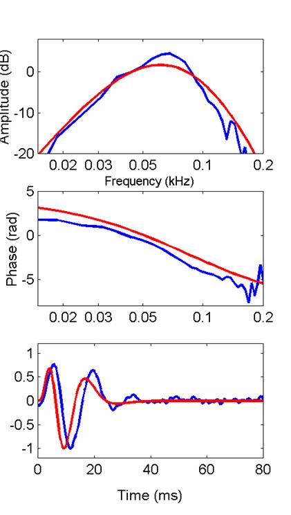
Mark was correct; we achieve a better fit to the filter function and its Bode plot with slightly higher order. One feature that the cascade of compartments cannot match is the near-periodicity in the filter function’s zero crossings. Notice in the model’s response that the zero- crossing intervals increase conspicuously as time progresses (a feature some investigators call a frequency glide). That generally seems not to be the case for saccular filter responses (they don’t glide as much). The near periodicity of the saccular filter function would lead as well to its slightly narrower and more peaked amplitude-Bode plot. We see the same features, to even greater degree in bullfrog AP and BP filter functions (see below).

• Model II gives us the narrowest tuning curve we can get with passive compartments (leaky integrators) alone.

• To match the bullfrog saccular, AP and BP data we evidently need to look elsewhere.

• Circuit theorists traditionally consider three kinds of elements (R, L, C).

• Compartmental models are equivalent to two-element (R,C or R,L) circuits.

• Now we’ll add the third element- - - giving us one more type of response . . . under-damped resonance.

• The impulse responses of highly under-damped resonances are not compact.

• Therefore, we’ll focus on slightly under-damped resonances.

b. RLC circuit models

Twentieth-century circuit theory had two complementary subfields- - circuit (network) analysis and circuit (network) synthesis. Among the important messages one derived from network synthesis, there is one especially appropriate to our situation here: for any linear transfer relation (such as our filter functions) there is an infinite number of realizations (different ways to achieve it, physically). Thus, no matter how well its behavior fits the data, a specific circuit model must be considered an affirmation of the consequent. Therefore, we need not consider specific circuit models here. All we must do is consider the newly available response type (slightly under-damped resonance) to see if it can compensate for the deficiencies of the compartmental model.

A

Filter functions for cascades of identical, slightly
under-damped resonances

Notice that in the higher-order filter functions, the zero-crossings are much more evenly spaced than they were in the compartmental models. This definitely is a step in the right direction. With appropriate combinations of compartmental processes and slightly under-damped resonances, we should be able to synthesize our frog inner-ear filter functions. The main point here is that we cannot do it with compartmental processes alone, something must be added.

Here are Bode plots for the four filter functions in figure A.

B

Note how different the Bode plots in B are from those in C, which are for a single resonance with various degrees of damping. None of our frog filter functions yielded amplitude Bode diagrams with concave flanks, such as those in C. The only abrupt phase shifts we found were in a subset of saccular units at anti-resonances (as opposed to resonances); those anti-resonances disappeared when the same saccular units were stimulated with airborne sound rather than substrate-borne vibration.

C

Each resonance comprises two separate integrating processes- - one accumulating potential energy, the other accumulating kinetic energy.

In a cascade of resonances, therefore, regardless of the degree of damping,

• Each resonance in the cascade adds 2 (12 dB/oct or 40 dB/dec) to the sum of the magnitudes of the asymptotic slopes in the Bode plot.

• Each resonance adds p radians (180 deg) to the phase range.

Conclusion to this point

With respect to band-pass filter functions from the bullfrog sacculus, AP and BP . . . .

• Our results, from dozens and dozens of units, suggest cascades of slightly under-damped resonances (possibly combined with leaky integrators).

• Our results are inconsistent with filters comprising single (or a few), more-highly under-damped resonances.

• Those are the principal strong inferences so far from these studies of Bode plots.

• We cannot infer how the resonances arise.

________________________________________

1.

• They could arise from combinations of complementary passive reactive elements analogous to L’s and C’s in electronics (e.g., masses combined with elastic elements).

2.

• They could arise from combinations of leaky integrative elements (such as first-order chemical reactions and compartmentalized diffusion processes) and feedback with active transducers (such as gated ion channels- - - as in the electric resonance model of R.S. Lewis & A.J. Hudspeth).

• Which would be analogous to phase-shift oscillators in electronics.

Note: The Lewis/Hudspeth resonance has been strongly inferred in

bullfrog saccular hair cells and in low-frequency hair cells from the

bullfrog amphibian papilla. This makes it the model of choice as we

attempt to account for the filter functions associated with those

hair cells. Occam’s razor trumps affirmation of the consequent; or,

Occam’s razor plus affirmation of the consequent yield strong inference.

3.

• Or, they could arise from combinations of leaky integrative elements and Onsager’s missing passive transducer– the anti-reciprocal transducer (or gyrator).

• With a cascade of leaky integrators alone, signal energy can flow only in the direction away from the input.

• In the three cases cited above, signal energy can bounce back and forth– flowing toward the input as well as away from it. This gives rise to the characteristic ringing of the under-damped system.

• The amplitude Bode plots for bullfrog saccular, AP and BP filters implies that there is some of this back-and-forth bouncing in each of those filters.

4. Dynamic order of bullfrog filters

The dynamic order of a circuit is given by the number of independently functioning Ls and Cs, or their equivalents, or, equivalently, by the number of separate leaky integration processes plus twice the number of separate resonances. For our experimental Bode plots, it is equal to or greater than the sum of the magnitudes of the asymptotic slopes.

For our saccular filter function, with its dynamic order of at least eight, we infer the following:

• Between the input point and the point of observation . . . .

• Bode plot implies a cascade of n slightly under-damped resonances plus m leaky integrators, where m +2n equals at least eight

• with at least three stages of differentiation.

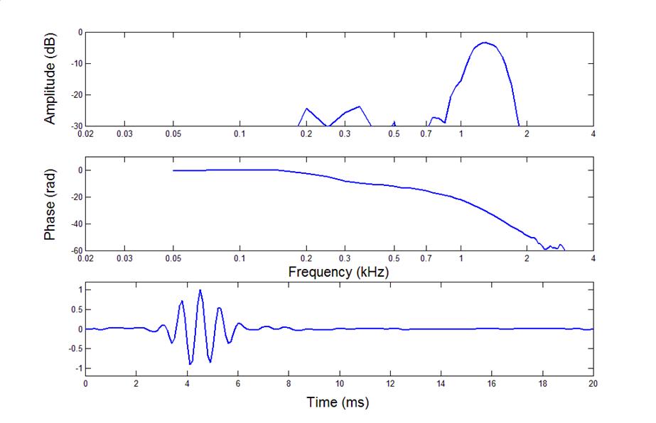
Here is a filter function from a bullfrog AP unit

• Between the input point and the point of observation . . . .

• Bode plot implies a cascade of n slightly under-damped resonances plus m leaky integrators, where m +2n equals at least ten to twelve

• with at least six stages of differentiation.

Here is a filter function from a bullfrog BP unit

• Between the input point and the point of observation . . . .

• Bode plot implies a cascade of n slightly under-damped resonances plus m leaky integrators, where m +2n equals more than twenty

• with more than ten stages of differentiation.

Here are filter functions from two bullfrog lagenar units

(from Kathy Cortopassi)

Here is the distribution of dynamic order in bullfrog lagenar units,

estimated from their Bode plots

(from Kathy Cortopassi)

• Between the input point and the point of observation . . . .

• the Bode plots imply a cascade of n slightly under-damped resonances plus m leaky integrators, where m +2n equals the dynamic order given in the figure.

• Bode plots for the low-pass filters imply no differentiation.

• Bode plots for the band-pass filters imply various numbers of stages of differentiation (four or five for the Bode plot in the right-hand panel above).

.

Further Conclusions

Whether they are taken from the bullfrog sacculus, the bullfrog amphibian papilla, or the bullfrog basilar papilla, the acoustic filter functions of the bullfrog inner ear reflect very high dynamic order, implying large numbers of separate integrative processes, in cascade, between the point at which stimulus is applied (external ear canal for AP and BP) and the point at which observations are made (VIIIth-nerve afferent axon). The dynamic orders of acoustic (band-pass) filter functions observed in the bullfrog lagena are moderately high- - distinctly higher than those of the vestibular (low-pass) filter functions from that same sensor. See Cortopassi & Lewis, 1998, for further discussion of the differences between acoustic and vestibular filter functions- - this was the theme of Kathy Cortopassi’s doctoral dissertation.

Bottom Line . . .

• However they arise, the acoustic filter functions of the bullfrog ear are beautiful . . .

• with compact, often nearly symmetric, impulse responses

• and very steep band edges- - -

• these are exactly what are required for very-high-resolution spectrographic analysis.

Footnote:

As filter functions are designed for increasingly sharp tuning, being symmetric and compact minimizes the distortion they impose on temporal waveforms. We can go back to our resonant filters for examples.

Here again are the filter functions formed by cascades of one, two, four and eight very slightly under-damped resonance (whose impulse response is depicted in the top line).

Here are the responses those filter functions would produce when the input waveform is the stimulus depicted in the top-most line, a tone burst at the filters’ BEF.

Notice that even with eight stages in cascade (dynamic order 16)

the distortion of the envelope of the stimulus waveform is relatively

minor, comprising largely finite rise and fall times and slight time delay.

Here again are the DFTs (Bode plots) of filter functions for a single resonance as it becomes increasingly under-damped.

Here are the responses those filter functions would produce when the input waveform is the

stimulus depicted in the top line, again a tone burst at the filters’ BEF

As the filter’s tuning becomes sharper, its temporal response becomes more sluggish.

These examples illustrate the chief advantage of a filter with high-dynamic order (many stages in cascade) over a filter comprising a high-Q, single-stage under-damped resonance. The fact that we see the former and not the latter in turtle, gerbil and bullfrog inner-ear acoustic senses is not surprising.

Epilogue

As I conclude this web page (on 03/27/2009), the biophysical circuitry underlying the peripheral filters of the bullfrog acoustic sensors remains largely unknown. On the other hand, the hearing research community has become increasingly comfortable with two elements that evidently are part of that circuitry in saccular units and in lower-frequency units of the amphibian papilla. One is electrical resonance in the individual (isolated) hair cells; the other is hair-bundle motility. The former has been demonstrated to include active elements- namely gated channels; the latter may or may not be an active process. The frequency distribution of the electrical resonances in AP hair cells matches very well that found in whole units. After the early observations of the resonances in saccular hair cells, this did not seem to be the case there. The resonant frequencies seemed too high. More recent observations show that they do fall into the correct range.*

It is very difficult for me to believe that occurrence of those resonances is coincidental. It seems that they must be participating in the tuning of the filters. They exhibit dynamic order two. The saccular filters and the low-frequency AP filters exhibit dynamic orders of eight or more. Furthermore, the range of phase shift and the slopes of the band edges displayed in Bode plots from those filters set a key constraint on the underlying biophysical circuitry—the eight or more integration processes implied by those high dynamic orders must be in cascade between the point of stimulus input and the point of spike triggering. In other words, parallel connection by a nerve fiber to four resonant hair cells will not suffice. If filtering in sacculus and low-frequency part of the AP depend solely on those resonances, then the resonances must be connected in cascade. What would be needed for that sort of connection is reverse transduction in the hair cells (hair-bundle motility driven by the electrical resonance). This was clear even before reverse transduction had been observed in non-mammalian vertebrates (Lewis, 1987). In the earlier discussions of reverse transduction, it was proposed as a device to reduce damping in the cochlea. In the bullfrog, it was and is needed for something very different; it is needed to link resonances into a cascade chain—thus providing peripheral filters with spectral resolution made high by steep band edges rather than sharp resonances.

That sounds simple. We now have the resonances, and we now have the reverse transduction. But how do we link them? Suppose we had a cascade chain of four hair cells, with input to the first one, output from the last one. That would give us the sort of Bode plots we’ve observed in the actual units. But how is the input limited to the first hair cell and the output limited to the last? Nothing seen so far in the saccular or AP micro-morphologies suggests answers to that question.

Considering mechanical elements only, which seems to be the entire story in higher-frequency AP units, Ellen Leverenz and I addressed the same sort of question in 1983. We couldn’t answer it then, and I don’t see an answer to it now. But the answer must be there, someplace. Considering the AP tonotopy we had just found, along with AP frequency-threshold tuning curves we obtained while doing that, we had surmised that AP tuning (filtering) was accomplished by some sort of traveling-wave process. What we were looking for in the AP micro-morphology, and did not find, was micromechanical underpinning for such a process. We were left with the conjecture that it somehow resided in the tectorial membrane.

*I thank Mark Rutherford for pointing this out to me.