The bullfrog sacculus:
from the outside
(Notes and figures from a seminar given at UCSF Sep. 2007)
Part 1
Context![]()
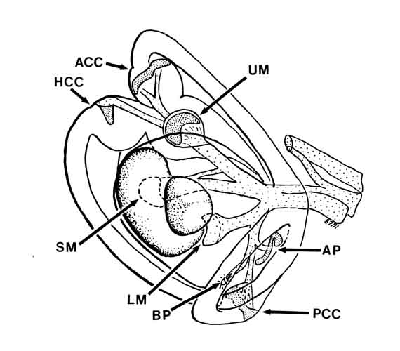
The saccular macula is one of eight sensory surfaces in the bullfrog inner ear. This drawing by Steve Myers shows the layout of those surfaces within the labyrinth. The meaning of most the labels should be self-evident to anyone familiar with the vertebrate ear. Three of the surfaces (basilar papilla {BP}, amphibian papilla {AP}, and saccular macula* {SM}) are devoted exclusively to acoustic sensing. A fourth (lagenar macula {LM}) is shared between the senses of balance and acoustic sensing. Acoustic sensitivity on the lagenar macula is confined to the centermost rows of hair cells. The spectral sensitivities are divided roughly as follows:
SM: 20-100 Hz
AP: 100-1000 Hz
BP: 1350 Hz
LM: 20-500 Hz
* In mammals, the saccular macula is devoted exclusively to the sense of balance.
Here are six amplitude Bode plots that illustrate the distribution of spectral sensitivity. Each was derived from triggered correlation between non-repeating broad-band noise stimuli and spikes from a single unit (blue = basilar papillar; green = amphibian papillar; red = saccular). The original data were taken in the Lewis Lab by Xiaolong Yu and Walter Yamada.
The bullfrog amphibian papilla appears to be a general auditory sensor—especially sensitive to air-borne sound, secondarily sensitive to substrate vibration. It is tonotopically organized along its S-shaped surface.
The basilar papilla is tuned to a dominant spectral component of the bullfrog vocalization. This is true generally for anurans, but the frequency of that component often places the best frequency (BEF) of basilar-papillar units far above the upper limit for the amphibian papilla—leaving a large gap in acoustic tuning.
The bullfrog saccular macula is primarily sensitive to substrate vibration, secondarily sensitive to air-borne sound. Its spectral sensitivity covers the three octaves immediately below the bottom of the amphibian papilla’s range.

Here I’ve added a Bode plot for a lagenar unit. The triggered-correlation data were taken by Kathy Cortopassi.
Triggered Correlation 1
First-order Wiener kernel
(de Boer’s REVCOR function)
The result of convolving the first-order Wiener kernel, h1(t), with a stimulus waveform, s(t), is a prediction of the time course of the linear (phase-locked) contribution to the instantaneous spike rate response to that stimulus.

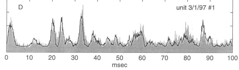
Here is a figure from Walter Yamada. The smooth trace in C is a filtered noise waveform, with a flat spectrum from 70 Hz to 600 Hz. It was applied repeatedly as auditory stimulation for an amphibian-papillar (AP) unit with BEF (best excitatory frequency) = 230 Hz. The resulting PSTH (instantaneous spike rate as a function of time) is the raggedy plot along the baseline. Note that the PSTH is not phase-locked to the stimulus waveform: in some places PSTH peaks correspond to peaks in the stimulus waveform; in other places they correspond to troughs.
The smooth trace in D is the result of convolving the stimulus waveform in C with the first-order Wiener kernel for this AP unit. Note how well it predicts the peaks and troughs in the PSTH.
Linear Filtering
One would apply the same operation (convolution) to construct a filtered version of a waveform:
f(t) = filter function s(t) = input waveform
r1(t) = ∑τ f(τ)s(t-τ) = conv [f(t), s(t)]
r1(t) = response of filter to s(t) ≡ the filtered version of s(t)
conv [ ∙ ] is a commutative operation
The fidelity of the prediction in the previous figure, which is comparable to that found over and over again by many investigators (beginning with de Boer & de Jongh) for low-BEF auditory units, tells us that the first-order Wiener kernel is a good approximation to such a unit’s peripheral filter function.
f(t) ≈ h1(t)
Furthermore, we see that the linear (ac) response of such a unit is phase locked to the filtered version of the stimulus, not to the stimulus itself.
Computation of the 1st-order Wiener kernel fails for high BEF units
Frequently, for such units,
f(t) ≈ SV1 [h2(t)]
where SV1 is the highest-ranking singular vector of the 2nd-order Wiener kernel, h2(t). For low-BEF units, the two functions usually are the same - - -
f(t) ≈ h1(t) ≈ SV1 [h2(t)]

Here is an example of the situation. These plots were derived from Walter Yamada’s data for AP unit 042895-7, whose BEF was close to 300 Hz. SV1 for the 2nd-order kernel is plotted in blue; the 1st-order kernel is plotted in red. Both functions yield essentially the same estimate of the peripheral filter.
Triggered Correlation 2
2nd-order Wiener kernel
Conv2 [h2(t), s(t)] = ∑τ1∑τ2 h2(τ1, τ2)s(t-τ1) s(t-τ2) yields estimates of 2nd-order distortion in the phase-locked (ac) response.
Conv2 [h2(t), s(t)] also yields estimates of positive and negative dc responses.
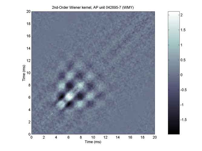
Here is the 2nd-order Wiener kernel for the same 300-Hz AP unit. It is a 200x200-element matrix of triggered autocorrelation values (derived from the segments of noise stimulus that occurred immediately prior to spikes). Note that white represents positive values, black represents negative values.
To separate components representing ac and positive dc responses from those representing negative dc responses, we decompose the 2nd-order Wiener kernel into an excitatory subkernel and an inhibitory subkernel.

Here is the excitatory subkernel. Again, white corresponds to positive values, black to negative values. Note the checkerboard pattern with a hint of background lines parallel to the main diagonal, which is a line of positive values.
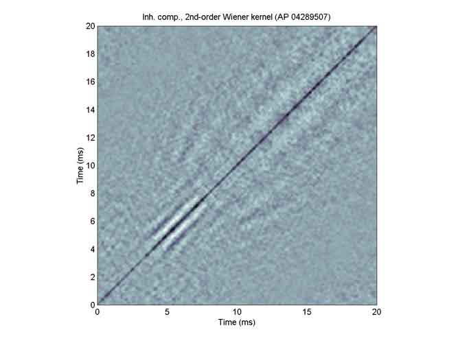
Here is the inhibitory subkernel. The main diagonal consists of negative values, and the patterns seem to comprise lines that are parallel to that diagonal or are diverging from it.
Separating excitatory components
To separate patterns representing ac response contributions from those representing positive dc contributions, we find the quadrature mate of SV1 (usually it’s SV2) and we compare the eigen value of SV1 to that of SV2.
Here are SV1 and SV2 for our 300-Hz AP unit. Note that SV2 (green) is 90-degrees out of phase with SV1 (red). This makes the two waveforms a quadrature pair. If these waveforms were less noisy, and if we squared each of them and summed the results, all of the gaps would be filled smoothly and we would be left with the square of the envelope of each of them- - - as in sin2() + cos2().
Here are the eigen values, k1 and k2, of SV1 and SV2 respectively. The corresponding contributions to the estimated second-order response given by the 2nd-order term in the Wiener series are - - -
rSV1 = k1 conv2 [SV1(t), s(t)] = k1 { conv [SV1(t), s(t)]}2
and
rSV2 = k2 conv2 [SV2(t), s(t)]
In the 2nd-order term in the Wiener series, these contribution combine by summation - - -
rcomb = rSV1 + rSV2
The combination yields two parts - - -
rcomb = (k1 – k2) conv2 [SV1(t), s(t)] + k2 {conv2 [SV1(t), s(t)] + conv2 [SV2(t), s(t)]}
The first part can be recognized as an estimate of the 2nd-order ac distortion contributed by SV1.
The second part is the sum of the squares of two filtered waveforms. Because the filter functions are in quadrature to one another, so too are the filtered waveforms—and the two of them have essentially the same envelope. The sum of their squares will yield the square of the envelope of either of them - - - which is the square of the envelope of the stimulus waveform filtered by our estimate of the unit’s peripheral filter function, f(t).
In general, the second part will not be dc. It frequently is given that name because it becomes dc (constant over time) when s(t) is a tone of constant amplitude.
It is instructive to look at the contributions of SV1 and SV2 to the excitatory subkernel.
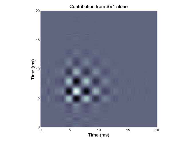

One can see that the essence of the excitatory subkernel is captured in one singular vector and its quadrature mate. This happens frequently.
These results generalize to - - - -
Rules of thumb for 2nd-order Wiener kernels
A checkerboard pattern corresponds to 2nd-order distortion of the ac (phase-locked) response component.
A pattern of parallel diagonal lines in the excitatory subkernel corresponds to a positive dc response component.
A pattern of parallel diagonal lines in the inhibitory subkernel corresponds to a negative dc response component.
Now we have a set of tools for looking at bullfrog acoustic sensors from the outside. We can add one more - - - Because it comprises triggered autocorrelation functions, the 2nd-order Wiener kernel can be converted easily to a map of the spectro-temporal receptive field (STRF).
Example
The bullfrog basilar papilla
(From Walter Yamada’s data)
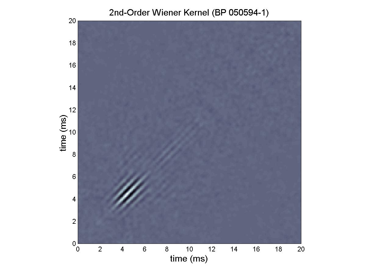


Walter found little variation in the second-order kernels of basilar papillar units. This unit, 050594-1 is thoroughly representative of them all. Note that the filter function, f(t), estimated by SV1, is beautifully symmetric—the sort of high-dynamic-order filter function that might be designed by a master electrical engineer to preserve temporal resolution while providing the desired spectral filtering. Although its units seem to be tuned to a common BEF, the basilar papilla of the adult bullfrog is not a simple sensor—its filter functions are far too elegant to be given that label.
The following two figures show, for another of Walter’s bullfrog BP units, how well the combination of SV1 and its quadrature mate can predict the PSTH in response to a repeated complex stimulus waveform.

The upper waveform in each of the panels above is that of a segment of band-limited noise, flat from 600 Hz to 3200 Hz. It was presented 6392 times as the PSTH displayed along the baseline in each panel was taken (from Yamada & Lewis, 1999).
Here is the same PSTH, along with the PSTH (dark line) predicted with the quadrature pair, SV1 and SV2. Although the prediction misses in a few instances, its general fidelity makes one comfortable with the conclusions that SV1 indeed is a good estimate of the filter function in BP units, and that the instantaneous spike-rate response indeed is predicted well by the square of the envelope of the filtered stimulus waveform.
Note about quadrature pairs of singular vectors
If one were to construct a sandwich model, comprising a high-BEF band-pass filter, followed by a square-law nonlinearity, followed by a low pass filter whose pass band did not overlap with that of the high-BEF band-pass filter, followed by a spike trigger model, and if one were to apply broad-band Gaussian noise as an input to the model and compute the 2nd-order Wiener kernel of the sandwich model by triggered correlation, the resulting kernel would yield a quadrature pair of singular vectors with equal eigen values. One of those vectors would be a close match to the impulse response (filter function) of the high-BEF band-pass filter; the other would be its quadrature mate (see Lewis and van Dijk, 2003).
The quadrature mate should be viewed simply as a mathematical construction-- representing the action of the sandwich model.
Note about singular-value decomposition and construction of subkernels
At the end of Part 2 of this presentation are m-files for carrying out these operations in MATLAB. Singular-value decomposition is executed in MATLAB with a single command.
Applying these tools to the four bullfrog acoustic sensors - - -
we find the following response properties - - -
Basilar papilla
Excitation
Positive dc response for stimulus frequencies in the neighborhood of BEF (1350 Hz)
Adaptation
Delayed negative dc response for the same stimulus frequencies

Here is a map of the spectro-temporal receptive field of Walter’s BP unit 050594-1. It was derived directly from the 2nd-order Wiener kernel. The method is described in Lewis & van Dijk, 2002; and the m-files for carrying out the process in MATLAB are given at the end of this presentation. The light blue background represents the mean power-spectral density of the noise stimulus used for triggered correlation. Darker blue shows spectro-temporal regions, prior to each spike, where the power-spectral density of the noise was below that mean level, the warm colors show spectro-temporal regions, prior to each spike, where the power-spectral was above that mean. In other words, when a spike occurred, the power spectral density approximately 4-6 ms earlier, in the vicinity of 1350 Hz had been (on average) conspicuously higher than its usual value; and the power-spectral density approximately 7-10 ms earlier, in the same spectral region, had been (on average) somewhat lower than its usual value. At the time of the spike (0 ms) a prior stimulus corresponding to the spectro-temporal region of the darker-blue patch would produce a moderately weak negative dc response, and a prior stimulus corresponding to the spectro-temporal region of the warm-color patch would produce a strong positive dc response. The latter corresponds to excitation of the unit; we presume that the former corresponds to what usually is called adaptation.
Amphibian papilla
Excitation
Variously distorted ac response for frequencies in the vicinity of BEF
(at higher BEFs the ac response becomes weak)
Positive dc response for the same frequencies (at higher BEFs the positive dc response dominates)
Adaptation
Delayed negative dc response for the same frequencies
Suppression
Negative dc response for stimuli coincident with excitatory stimuli, but at higher frequencies

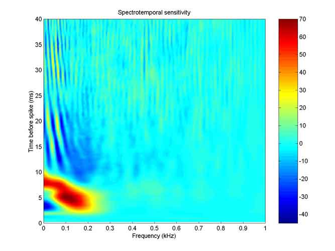
Here is a map of the spectro-temporal receptive field of Walter’s AP unit 042895-7, the same 300-Hz unit we were examining earlier. The excitatory (warm-colored) patch represents both ac distortion and positive dc response. From the difference between the eigen values of SV1 and SV2, about 75% reflects distortion, 25% reflects positive dc (envelope-squared) response.
The blue patch lying above the excitatory patch is most reasonably interpreted as reflecting adaptation. The two blue patches to the right of the excitatory patch undoubtedly reflect suppression. All of these negative effects can be interpreted directly from the inhibitory subkernel. Time in the STRF is measured along the main diagonal in the 2nd-order kernels and subkernels. Thus, the 10-ms point corresponds to x=10 ms, y=10 ms along the diagonal of the inhibitory subkernel. The blue patch between 700 and 1000 Hz corresponds to the patch of parallel diagonal lines centered around the 6-ms point in the inhibitory subkernel. The darker blue patch, just to the right of the excitatory patch, corresponds to the lines that diverge from the main diagonal in the vicinity of the 8-ms point in the inhibitory subkernel. The blue patch directly above the excitatory patch corresponds to the large patch of parallel diagonal lines centered around 15 ms in the inhibitory subkernel.
All of the blue patches represent negative dc (square-of-the-envelope) responses. These images allow us to see their relative timing as well as their spectral sensitivities. They also demonstrate that all of these inhibitory effects are at play when the AP is stimulated by complex acoustic waveforms. The importance of the square-law relationship will become clearer when we compare AP responses to saccular responses.
Lagena
Excitation
Variously distorted ac response over a very broad pass band
Adaptation
Delayed negative dc response for the same frequencies
Here is a map of the spectro-temporal sensitivity of Kathy’s lagenar unit 060794-2A.
Sacculus
Excitation
Variously distorted ac response over the pass band
Adaptation
Occasionally, delayed negative dc response over the same frequencies
Generally, the 1st-order kernel tells the whole story

Here is the 1st-order Wiener kernel for Xiaolong’s saccular unit 011590-20. The band-edge slope on the left side of the Bode amplitude plot is approximately 12 dB/oct, that on the right is approximately -24 dB/oct. This combination implies dynamic order six (6 times 6 dB/oct) or greater for this unit. When we first began studying bullfrog saccular physiology, we obtained Bode plots with point frequency observations.

Here is such a Bode plot that Ellen Leverenz and I constructed in 1983. The sum of the magnitudes of the band-edge slopes in this case is 42 dB/oct, implying dynamic order seven or greater. The points were obtained with discrete Fourier transformation applied to cycle histograms.
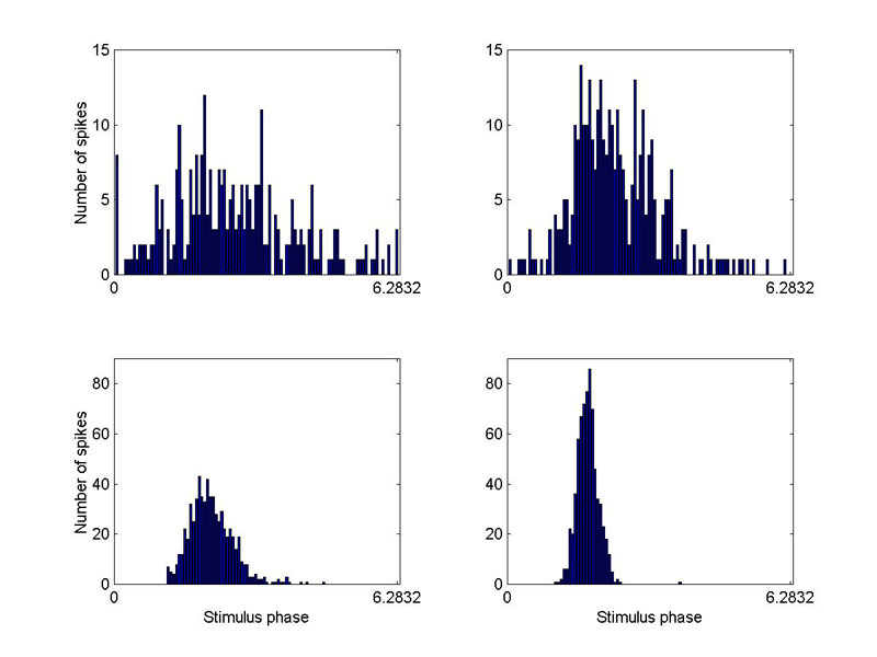
Here are four cycle histograms taken by Ellen and me in 1981 (unit 110381-5). The stimulus was a 70-Hz sinusoidal vibration applied along the dorso-ventral axis of the bullfrog. The peak amplitude of the stimulus for the upper left-hand graph was 0.01 cm/s2, for the upper right it was 0.02 cm/s2, for the lower left -- 0.07 cm/s2, and for the lower right -- 0.2 cm/s2. A full cycle of phase (0 to 2π rad) is represented along the horizontal axis. Note that the modulation of instantaneous spike rate in the upper left-hand graph is nearly sinusoidal, reflecting nearly linear response. For lower stimulus levels, it became even more so. To compute a unit’s gain, we used such low stimulus levels and collected a fairly large number of spikes. Then we applied discrete Fourier transform to the cycle histogram to obtain an objective estimate of the peak instantaneous spike rate in the fundamental frequency component. Dividing by stimulus amplitude gave us the estimate of gain. As we soon shall see, we need not have gone to so much trouble. Linearly-responding units were robustly so – over very large ranges of stimulus amplitude.
What’s Special about the Bullfrog Sacculus?
In terms of signal processing, the bullfrog sacculus seems pretty dull. Is there anything special about it- - - other than the fact that its hair cells have been studied more than those of any other inner-ear organ?
Answer: It has the greatest sensitivity to seismic stimuli (substrate vibration) yet found in any terrestrial animal, exhibiting clear single-unit responses to vibration amplitudes well below 0.01 cm/s2 (RA Baird, H Koyama, EL Leverenz, ER Lewis).
The previous champs were snakes (P Hartline) and cockroaches (Autrum & Schneider), both of which exhibited thresholds of approximately 0.02 cm/s2.
More to come - - - - in Part 2