Compiling Computational Graphs

Stochastic Computational Graphs provide efficient intermediate representations for expressing canonical families of neural networks. As a graph, the nodes are operators with tensors as edges. Operators for expressing architectures such as ResNetsDeep residual learning for image recognition, He et al, 2016, TranformersAttention is all you need, Vaswani et al, 2017 include complex operators such as Convolutions, Attention, etc.

It turns out that composing such operators (or chains-of-operators) in specific ways is amenable to tractable optimization via gradient descent algorithms. However, designing systems that scale gracefully across clusters of (heterogeneous) devices present several challenges. Moreover, the hierarchical nature of these computational graphs introduces dependencies that induce tradeoffs such as resource utilization (throughput) vs. model capacity. While there are multiple ways of dissecting this tradeoff, let's start with the most obvious ones:

1. orchestrating the placement of nodes
2. storage, communication of edges

Table of Contents

1. SCGs: Abstractions for Representing Neural Networks
2. Case Study : Transformers
3. Distributing Computation by Graph Partitioning
4. Implementing Sharding Strategies
5. Automating Distributed Trainings
6. Open Questions

SCGs: Abstractions for Representing Neural Networks

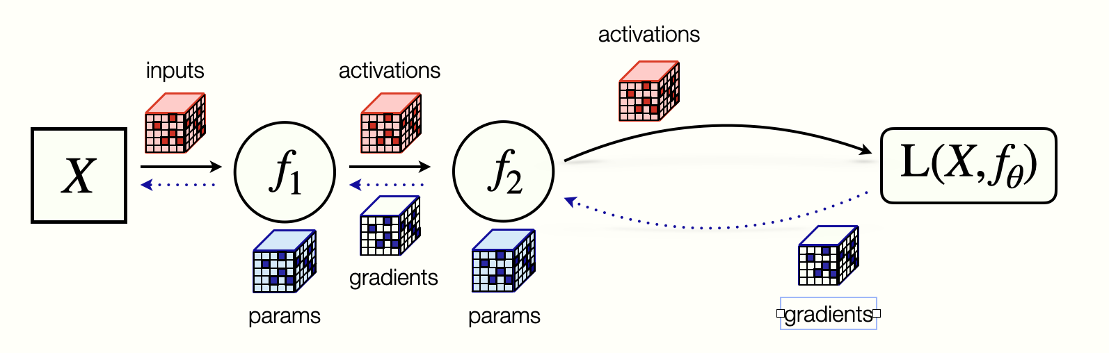
Broadly, neural networks are implemented as a directed acyclic graph (DAG), composed of complex operators and tensors. Training wih learning algorithms such as gradient descent is typically two-phase (i) forward propagation (e.g. generating prediction) (ii) backward propagation (for updating parameters). The memory, storage, and computation requirements of a neural network depend on the structure and state of different subgraphs during each phase.

⊕Representing a neural network as a DAG, highlighting tensors and operators.

One abstraction to reason about implementing an SCG, defines tensor programs. Such programs are implemented via high-level languages or frameworks such as TensorFlow, PyTorch & JAX.

Neural Networks are stateful machines, distilling massive datasets into a relatively small number of parameters. As a principle, we separate out the concerns related to maintaining state, from the concerns related to computing. For illustration, let's implement a simple Multi-Layer Perceptron (MLP) JAX MLP example

        
          """
          implements a multi-layer perceptron
          """
        
          ## initialize all parameters of the model
          ## note: feature_dim per layer is a sufficient 
          ## program sketch for the weight tensors
          
          def init_network_params(hidden_layer_sizes, base_key):
              keys = random.split(base_key, len(hidden_layer_sizes))
              return [_mlp_random_params(
                          indim, outdim, key) for indim, outdim, key in zip(
                          hidden_layer_sizes[:-1], hidden_layer_sizes[1:], keys)]

          params = init_network_params(hidden_layer_sizes, random.PRNGKey(0))
        
          ## per-sample computation in forward pass 
          
          def predict(params, image):
              activations = image
              for w, b in params[:-1]:
                outputs = jnp.dot(w, activations) + b
                activations = relu(outputs)

              final_w, final_b = params[-1]
              logits = jnp.dot(final_w, activations) + final_b
              return logits - logsumexp(logits)

        
      

Case Study : Transformers

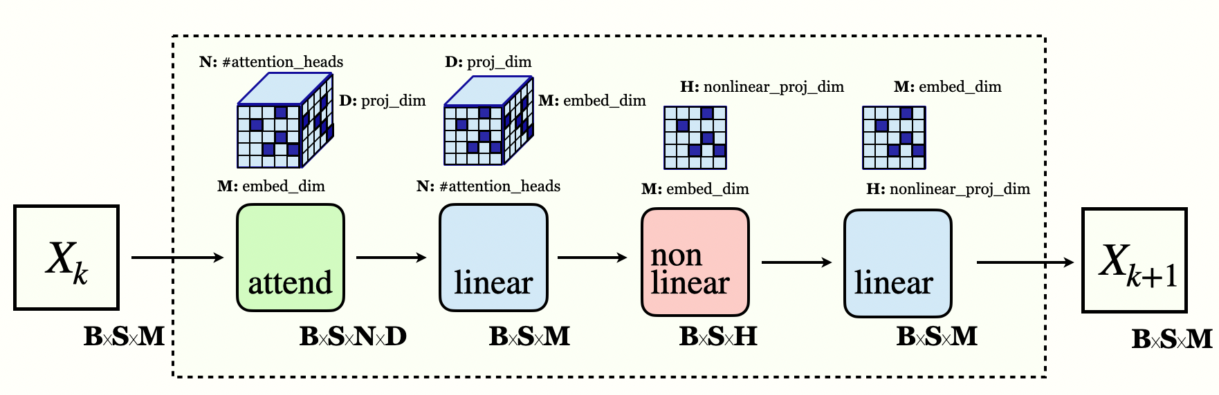
Transformers are neural network architectures, where multi-head attention (MHA) and non-linear projection layers are composed across multiple layers. A quick accounting of the parameters of the model, and memory requirements, reveals challenges in scaling the models, and PCGs in general.

Transformer Layer

⊕Data Parallelism introduces microbatches, where a batch is split across multiple devices to accomodate for large models.
Attention is all you need, Vaswani etal 2017

Distributing Computation by Graph Partitioning

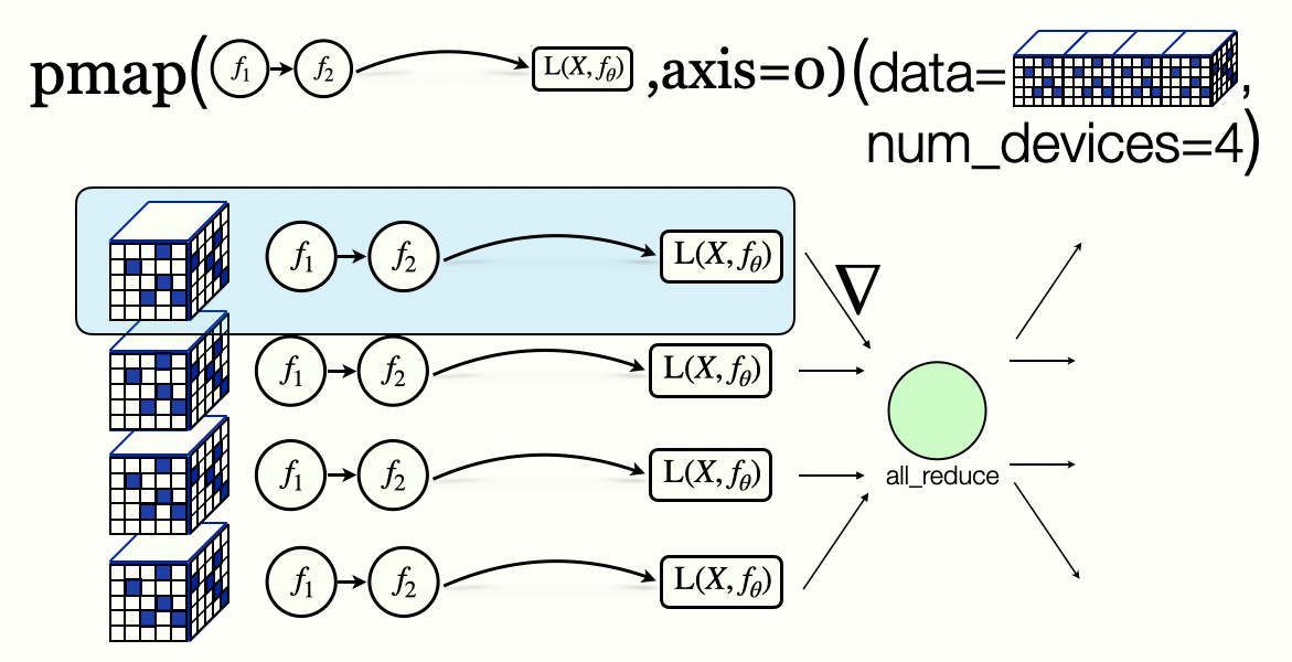
Data Parallelism

⊕Data Parallelism introduces microbatches, where a batch is split across multiple devices to accomodate for large models.
Imagenet classification with deep convolutional neural networks Krizhevsky etal 2012

Model Parallelism

⊕Model Parallelism partitions the PCG across multiple devices, introducing the notion of a pipeline, essential for GPT/PaLM scale models.
Megatron-LM: Training Multi-Billion Parameter Language Models Using Model Parallelism ,Shoeybi etal 2019

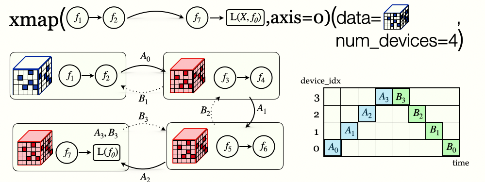
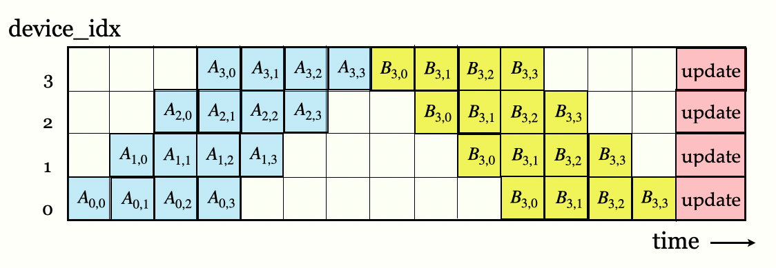
Pipeline Parallelism

⊕Pipeline Parallelism reduces underutilization, where a batch is split across multiple devices to accomodate for large models.
GPipe: Efficient Training of Giant Neural Networks using Pipeline Parallelism, Huang etal 2018

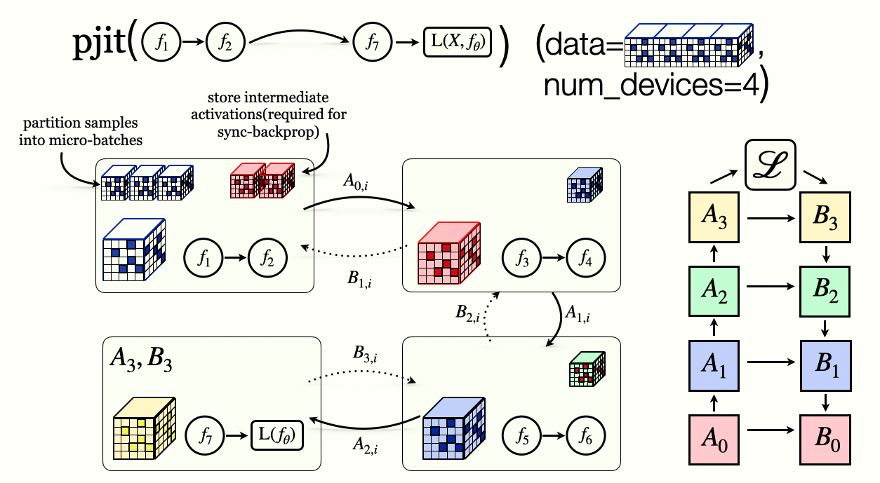
Implementing Sharding Strategies

Abstractions are useful when they hide the implementation details of the underlying system. In other words, a high-level program that works on a single device should generalize to multiple devices with minimal modifications.

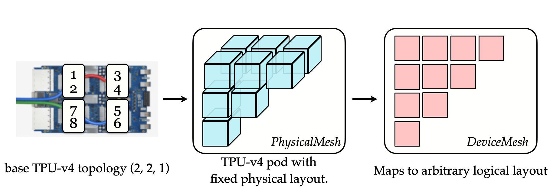
[It] takes in an XLA program that represents the complete neural net, as if there is only one giant virtual device.

To ground this idea of a large virtual device into implementation, JAX/XLA defines a DeviceMesh; a logical mesh outlining the available resources for certain computations. An instructive example is considering a TPU-style accelerator, where a single pod provides 4 chips with 2 cores each. This topology is mapped to a logical mesh of 4x2=8 devices, with partitions along two axes.

⊕A device mesh has different nodes interconnected with different levels of communication primitives.
JAX xmap tutorial

Now, implementing the various parallelism strategies require us to find ways of placing relevant operations onto the correspondin devices. All instances of parallelism we've discussed broadly fall into two categories:

1. Inter-Op parallelism: data-parallelism, model parallelism
2. Intra-Op parallelism: pipeline-parallelism

As noted above, the definition of the computation graph should ideally be abstracted away from the how it's implemented on different compute devices. To this effect, JAX/XLA annotate tensors with a sharding property, so that the XLA compiler can determine how to place operations.

⊕Compiling and partitioning operators and tensors.
GSPMD: General and Scalable Parallelization for ML Computation Graphs , Xu etal 2022

Automating Distributed Training

Building on the intuition of hierarchical parallelism, first at an inter-operator and then an intra-operator level, a natural question to ask is how to automatically generate the layouts of the various parallelism strategies.

⊕Given resource constraints, how do we generate and distribute operators efficiently?
Alpa: Automating Inter-and Intra-Operator Parallelism for Distributed Deep Learning, Zheng etal 2022

Open Questions