Generative Models 001

One view of machine learning is that it is the study of algorithms that make inference about probability distributions. In this view, the dataset is viewed as a sample from some underlying unknown probability distribution. That is for some unknown probability distribution $(P,\mathcal{X})$, defined on a set $\mathcal{X}$, we have a dataset $\mathcal{D}=\{x_1,\dots ,x_n\}$, where each $x_i\sim P$. Given samples from the unknown distribution, we can define different inference tasks that aim to reason about the underlying distribution. Some examples include:

• Density estimation: Given a dataset $\mathcal{D}$, estimate the probability density function $p(x)$ of the underlying distribution $P$.
• Data generation : Given a dataset $\mathcal{D}$, generate new samples from the underlying distribution $P$.
• Representation Learning : Given a dataset $\mathcal{D}$, learn a representation of the underlying distribution $P$. This is particularly useful for high-dimensional support we have limited annotated data.

Generative Models

We focus on three classes of generative models:

• Likelihood-based models Given a family of parametric models $\mathcal{M}$, we aim to learn a model $p_{\theta }$ from the family $\mathcal{M}$ that is close to the true distribution $p_{\mathrm{data}}$. This is done by maximizing the likelihood of the observed data under the model, i.e. $\underset{\theta }{max}{\mathbb{E}}_{x\sim p_{\mathrm{data}}}[\log p_{\theta }(x)]$
• Implicit models An alternative approach to representing a probability distribution, is to model the generative process. In other words, instead of explicitly modeling the density, we learn how to directly sample new points $\hat{x}\sim p_{\mathrm{data}}$. Note that with enough samples, we can estimate the density of the distribution by computing the empirical distribution ${\hat{p}}_{\mathrm{data}}$.
• Diffusion models An emerging class of generative models is $\mathit{\text{score-based}}$ or $\mathit{\text{diffusion}}$ models. Note that in likelihood-based models we care about ${\mathrm{\nabla }}_{\theta }\log p_{\theta }(x)$ that informs us about the direction of descent in the parameter space. In diffusion models, we instead care about the $\mathit{\text{score}}$ ${\mathrm{\nabla }}_x\log p_{\theta }(x)$ that informs us about how the inputs themselves should be perturbed to increase the probability of the output. Additionally, diffusion models are typically $\mathit{\text{iterative}}$ samplers, where the inputs are perturbed multiple times to generate an output.

Unsupervised Representation Learning

Consider the setting where you have access to large amounts of unlabelled images from the internet, $\mathcal{D}=\{x_1,\dots ,x_n\}$, where each $x_i\in {\mathbb{R}}^d$. How do we learn meaningful representations of the data?

Contractive Autoencoder

One approach is performing non-linear dimensionality reduction using neural networks. For example, with a $\mathit{\text{contractive autoencoder}}$, we learn an encoder $f_{\theta }(x):{\mathbb{R}}^d\to {\mathbb{R}}^k$ and a decoder $g_{\varphi }(z):{\mathbb{R}}^k\to {\mathbb{R}}^d$, such that $g_{\varphi }(f_{\theta }(x))\approx x$.

Denoising Autoencoder

As we've seen in lecture, data augmentations present a powerful tool for improving the generalization of neural networks. An instantiation of this in the autoencoder setting is the denoising autoencoder Extracting and Composing Robust Features with Denoising Autoencoder, Vincent et al 2008 . In this setting, we corrupt the input $x$ with noise $ϵ$ and learn an encoder $f_{\theta }(x):{\mathbb{R}}^d\to {\mathbb{R}}^k$ and a decoder $g_{\varphi }(z):{\mathbb{R}}^k\to {\mathbb{R}}^d$, such that $g_{\varphi }(f_{\theta }(x))\approx x$.

Comparing Distributions

One of the core objectives of generative models is to learn $p_{\theta }$ that is close to $p_{\mathrm{data}}$. This requires defining a notion of $\mathit{\text{closeness}}$ between two distributions. Consider the setting where we have two distributions $P(x)$ and $Q(x)$, that share the same support $\mathcal{X}$. Metrics that are commonly used to compare two distributions include:

• Kullback-Leibler Divergence: $\mathrm{KL}(P||Q)={\mathbb{E}}_{x\sim P}[\log \frac{P(x)}{Q(x)}]$
• Jensen-Shannon Divergence: $\mathrm{JS}(P||Q)=\frac{1}{2}\mathrm{KL}(P||M)+\frac{1}{2}\mathrm{KL}(Q||M)$, where $M(x)=\frac{P(x)+Q(x)}{2}$

Note that the KL divergence is generally asymmetric, i.e. $\mathrm{KL}(P||Q)\ne \mathrm{KL}(Q||P)$.

Variational Autoencoder

VAEs fall in the class of likelihood-based models. The goal is to learn a model $p_{\theta }(x)$ that is close to the true distribution $p_{\mathrm{data}}$. This is done by maximizing the likelihood of the observed data under the model, i.e. $\underset{\theta }{max}{\mathbb{E}}_{x\sim p_{\mathrm{data}}}[\log p_{\theta }(x)]$.

Evidence Lower Bound

Given a latent-variable model, $z\to x$, we have an alternative objective to maximize the likelihood of the data, i.e. $\underset{\theta }{max}{\mathbb{E}}_{x\sim p_{\mathrm{data}}}[\log p_{\theta }(x)]$. In particular, consider the expression $$\begin{array}{rl}\log p_{\theta }(x)& =\log {\int }_z{p}_{\theta }(x,z)\mathrm{d}z\\ & =\log {\int }_z{p}_{\theta }(x|z)p(z)\mathrm{d}z\end{array}$$ The above formulation, is equivalent to sampling $\mathit{\text{latent-variables}}$ $z$ from the prior $p(z)$ and then computing the likelihood of the data given the latent variables. However, when the latent-variables are continuous, estimating the above expression requires integrating over the entire latent space. As this is intractable in practice, we could instead sample a finite number of latent variables $z_1,\dots ,z_n$ from the prior $p(z)$ and then compute the likelihood of the data given the latent variables. This is known as the $\mathit{\text{Monte Carlo approximation}}$, where we approximate the integral with a sum: $$\begin{array}{rl}\log p_{\theta }(x)& \approx \log \sum _{i=1}^n{p}_{\theta }(x|z_i)p(z_i)\end{array}$$ Note that typically, for $x\in {\mathbb{R}}^d,z\in {\mathbb{R}}^k$ with $(k<d)$. Estimating the likelihood of the higher-dimensional data $x$ conditioned on the lower-dimensional latent-variables $z$ is unstable to train, due to high variance gradients. Instead we consider an alternative formulation, where we additionally want to find a paramteric approximation $q_{\varphi }(z|x)$ of the posterior distribution $p(z|x)$ of latents $z$ given observed datapoints $x$, This is known as the $\mathit{\text{variational inference}}$ framework. In particular, we have the following expression: $$\begin{array}{rl}\log p_{\theta }(x)& =\log {\int }_z{p}_{\theta }(x|z)p(z)\mathrm{d}z\\ & =\log {\int }_z\frac{q_{\varphi }(z|x)}{q_{\varphi }(z|x)}{p}_{\theta }(x|z)p(z)\mathrm{d}z\\ & =\log [{\mathbb{E}}_{z\sim q_{\varphi }(z|x)}\{\frac{p(z)}{q_{\varphi }(z|x)}{p}_{\theta }(x|z)\}]\mathrm{d}z\end{array}$$ Note that the above expression is valid for all approximations of the posterior $q_{\varphi }(z|x)$ as long as the support of $q_{\varphi }(z|x)$ is a superset of the support of $p(z)$. Optimizing the above expression is still difficult; instead we optimize a lower bound of the above expression, derived with help of Jensen's inequality.

⊕ Jensen's inequality for concave functions.

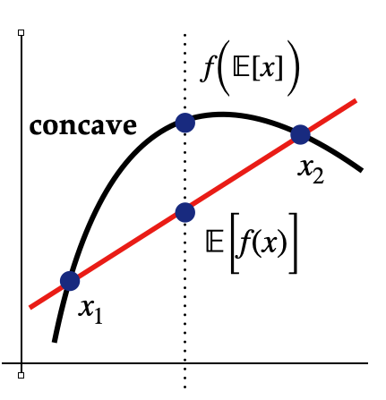
In particular, for any concave function ($\log$ in this case), we have the following inequality: $$\begin{array}{r}f(\mathbb{E}[x])\ge \mathbb{E}[f(x)]\end{array}$$ Plugging this inequality into the variational expression, we have the following lower-bound for true likelihood: $$\begin{array}{rl}\log p_{\theta }(x)& \ge {\mathbb{E}}_{z\sim q_{\varphi }(z|x)}\{\log \frac{p(z)}{q_{\varphi }(z|x)}{p}_{\theta }(x|z)\}\\ & ={\mathbb{E}}_{z\sim q_{\varphi }(z|x)}\{\log p_{\theta }(x|z)-\log \frac{q_{\varphi }(z|x)}{p(z)}\}\\ & ={\mathbb{E}}_{z\sim q_{\varphi }(z|x)}[\log p_{\theta }(x|z)]-{\mathbb{E}}_{z\sim q_{\varphi }(z|x)}[\log \frac{q_{\varphi }(z|x)}{p(z)}]\\ & =\underset{\text{Reconstruction Likelihood}}{\underbrace{{\mathbb{E}}_{z\sim q_{\varphi }(z|x)}[\log p_{\theta }(x|z)]}}-\underset{\mathrm{Matching}\mathrm{Posteriors}}{\underbrace{\mathrm{KL}(q_{\varphi }(z|x)||p(z))}}\end{array}$$ The above approximation is called the Evidence Lower BOund (ELBO) and is easier to optimizer in practice Auto-encoding variational bayes , Kingma & Welling 2013. One way to approximate the above expression is that we want to increase the likelihood of decoding the data given the latent variables, while also matching the posterior distribution of the latent variables to a distribution from which we can sample efficiently (e.g. Gaussian).

⊕ Sketch of the architecture design for Variational Autoencoders. Notably, the architecture admits a stochastic node.

Gradient based optimization of the above formulation is still difficult, since taking gradient through a stochastic node (e.g. sampling from a distribution) is not differentiable. To overcome this, we use the reparameterization trick to sample from the posterior distribution $q_{\varphi }(z|x)$, by sampling from a standard normal distribution and then transforming it to the posterior distribution. In particular, consider sampling from a Gaussian distribution $N(\mu ,{\sigma }^2)$, where $\mu$ and $\sigma$ are parameters of the distribution. Sampling from the original distribution can be reparameterized as follows: $$\begin{array}{r}ϵ\sim N(0,1)\\ z=\mu +\sigma \odot ϵ\end{array}$$ This resolves the trainability issue, since the above expression provides a modified computation graph:

Generative Adversarial Networks

As an implicit model, GANs present a different perspective to modelling the data distribution Generative Adversarial Networks , Goodfellow 2014. In particular, GANs are composed of two networks:

• Generator: $G_{\theta }(z):{\mathbb{R}}^k\to {\mathbb{R}}^d$, where $z\sim p(z)$
• Discriminator: $D_{\varphi }(x):{\mathbb{R}}^d\to \mathbb{R}$, where $x\sim p_{\mathrm{data}}(x)$

⊕ Sketch of GANs, admits adversarial training to enable sampling from data-distribution.

Training

The high level intuition behind training GANs is that we want to train the generator to create samples that are indistinguishable from the real data. At the same time, we want to train the discriminator to be able to distinguish between real and fake data. This presents the following $\mathit{\text{minmax}}$ optimization problem: $$\begin{array}{r}\underset{G_{\theta }}{min}\underset{D_{\varphi }}{max}\underset{\text{Real Samples}}{\underbrace{{\mathbb{E}}_{x\sim p_{\mathrm{data}}(x)}[\log D_{\varphi }(x)]}}+\underset{\text{Synthetic Samples}}{\underbrace{{\mathbb{E}}_{z\sim p(z)}[\log (1-D_{\varphi }(G_{\theta }(z)))]}}\end{array}$$

⊕ Jensen's inequality for concave functions.

Sampling

Sampling from GAN is done by sampling latents from the prior distribution $p(z)$ and then passing it through the generator network. In particular, we have the following generative process: $$\begin{array}{r}z\sim p(z)\\ x=G_{\theta }(z)\end{array}$$

Diffusion Models

The algorithms and models we've considered directly learn to either estimate density (VAEs) or generate samples (GANs). Notably, these algorithms are single-step, meaning that there is a single step of probabilistic inference (variational or implicit).

⊕ Diffusion models present iterative-samplers that incrementally walkback from a noisy distribution to realistic samples from data-distribution.

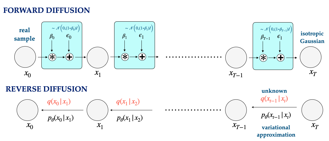
Diffusion models are a class of generative models that are $\mathit{\text{multi-step}}$, meaning that they perform multiple steps (say T) of inference. In particular, diffusion models are composed of two phases:

• Forward: In this phase, we start from samples from the real distribution and iteratively add noise to the samples. In particular, starting from $x_0\sim p_{\mathrm{data}}$ we have: $$\begin{array}{r}q({\mathbf{x}}_t|{\mathbf{x}}_{t-1})=\mathcal{N}(\sqrt{{\beta }_{t-1}}{\mathbf{x}}_{t-1},(1-{\beta }_{t-1})\mathbb{I})\end{array}$$ Notably, the variance of the distribution is a function of the step $t$, and the variance increases as we move forward in time. A typical example Denoising Diffusion Probabilistic Models, Ho 2020 of this would be linearly increasing from ${\beta }_0={10}^{-4}$ to ${\beta }_T=0.02$.
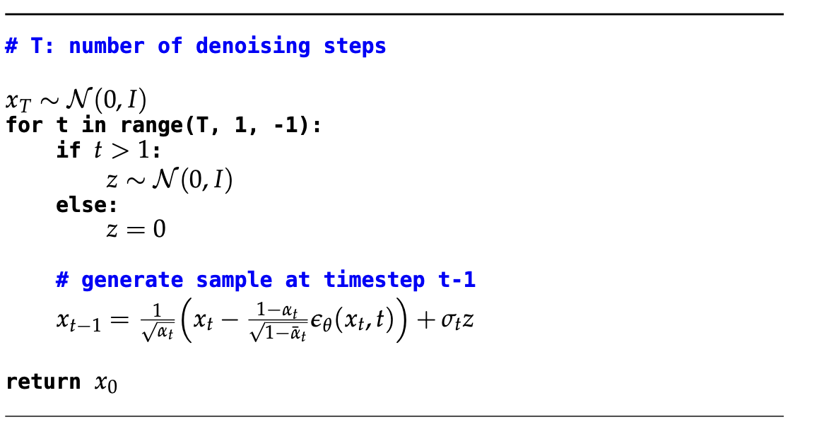
• Reverse: Sampling from the diffusion model is done by starting from a sample from our target distribution (e.g. isotropic Gaussian) and iteratively denoising the noisy inputs. In the Markov chain illustrated above this corresponds to starting at $x_T$ and moving backwards in time, such that $x_0$ is the denoised sample. Performing this denoising step, however requires us to estimate $q(x_{t-1}|x_t)$ which is not tractable. Instead, we perform a variational inference to estimate this posterior distribution, and maximize the ELBO (as in VAEs) for each time-step. A key insight that enables such inference, is that one can recover a closed form Denoising diffusion probabilistic models expression for $(x_{t-1}|x_t,x_0)$.

For more details on the diffusion model, we refer the reader to these wonderful blog posts Generative Modeling by Estimating Gradients of the Data Distribution, Song 2021 What are Diffusion Models?, Weng 2021.

Training

⊕ Training the score function for diffusion models

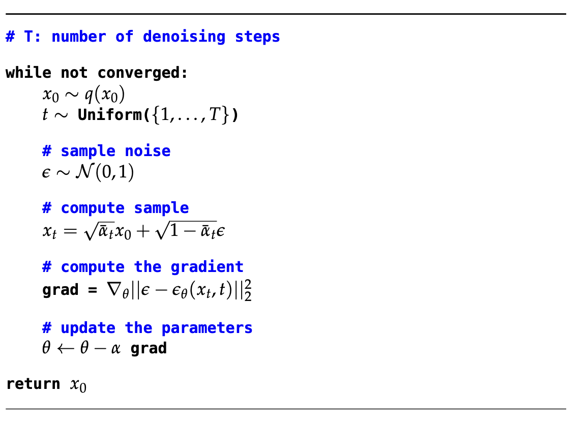
With a trained estimator for the score function, we can reverse the diffusion process to sample from the data-distribution.

⊕ Sampling from diffusion model.