| Date | Section | Change |
|---|---|---|
| 06/02/98 | ||
| Online Resources | Updated the pointer to A.T. Campbell's home page. | |
| 01/22/98 | ||
| Online Resources | Added a pointer to the Id Software source code and utilities (finally). | |
| 06/08/97 | ||
| Building a tree | Added definition of an autopartition. | |
| Efficiency | Completely rewrote this section with a concise explanation of the complexity of HSR with an autopartition. | |
| Online Resources | Updated link to Paton Lewis's BSP tree page, and added a link to Tom Hammersly's web page which describes his experience at implementing a BSP tree compiler and viewer. | |
| 06/01/97 | ||
| Motion Planning | Initial draft. | |
| Doom | Removed text which is confusing and not quite informative enough. Still looking for a replacement. | |
| 04/29/97 | ||
| Online Resources | Updated the link to the Computational Gemoetry Pages. | |
| 04/25/97 | ||
| What is... | Corrected an error in the ascii-art version of the tree diagram. | |
| Building BSP Trees | Corrected an error in the example code. | |
| 04/14/97 | ||
| Boolean Ops | Corrected an error: "... polygon EFGH is inserted ... one polygon at a time." was changed to "... is inserted ... one edge at a time." Thanks to Filip J. D. Uhlik for noticing this. | |
| 04/08/97 | ||
| Online Resources | Updated pointer to FTP site for the FAQ support files: ftp://ftp.sgi.com/other/bspfaq/. | |
| 04/02/97 | ||
| Entire Document | Moved document to reality.sgi.com. Changes were made to reflect the new host, but otherwise only a few minor HTML changes were made. | |
| 10/09/96 | ||
| Acknowledgements | Added a Michael Brundage to the acknowledgements. | |
| Online Resources | Added a reference to GFX, a general graphics programming resource. Added a reference to John Whitley's BSP tree tutorial page. | |
| 10/07/96 | ||
| Definitions | Added new definitions page to clarify some difficult terms. | |
| Ray Tracing | Added a note about using the parent node of the ray origin as a hint for improving run-time performance. | |
| Efficiency | Corrected a long standing error in the stated complexity of BSP trees for Hidden Surface Removal. | |
| 10/06/96 | ||
| About | Added new sub-sections describing the intended audience for the FAQ, and guidelines for obtaining assistance from the FAQ maintainer. | |
| Definition | Began to re-word the overview of BSP trees in an attempt to make the definition clearer. | |
| 08/21/96 | ||
| Online Resources | Added a reference to Paton Lewis's Java based BSP tree demo applet. | |
| 08/07/96 | ||
| Online Resources | Added a reference to the Win95 BSP Tree Demo Application. | |
| 07/24/96 | ||
| Online Resources | Added reference to Michael Abrash's ftp site at Id. | |
| 07/11/96 | ||
| Online Resources | Added reference to Andrea Marchini and Stefano Tommesani's BSP tree compiler page. | |
| 05/01/96 | ||
| General | The FAQ articles may now be annotated using the forum mechanism. | |
| 04/28/96 | ||
| Forum | Experimental new discussion area for BSP trees. | |
| 04/24/96 | ||
| General | Added "Next" and "Previous" links on each page of the FAQ. | |
| 04/17/96 | ||
| Whole FAQ | The web search engines have been pointing a lot of people at the entire listing version of the FAQ, rather than at the indexed version. This has led to significantly increased load on our server, and slow response times. As a result, I have made it possible to view the whole document only by following the link from the index page. | |
| 04/12/96 | ||
| Online Resources | Update on A.T. Campbell's resources | |
| 04/08/96 | ||
| Eliminating Recursion | Initial Draft with code example | |
| 03/25/96 | ||
| General | White pages | |
| 03/22/96 | ||
| Online Resources | A.T. Campbell's home page Update Mel Slater's location | |
| 03/21/96 | ||
| Contribution | Corrected e-mail address | |
| Online Resources | Arcball FTP site Paper by John Holmes, Jr. | |
| 02/19/96 | ||
| Changes | NEW | |
| Ray Tracing | Draft implementation notes | |
| Analytic Visibility | Draft contents | |
| Boolean Operations | Spelling corrections | |
--
Last Update: 09/06/101 14:50:28
General
The purpose of this document is to provide answers to Frequently Asked Questions about Binary Space Partitioning (BSP) Trees. The intended audience for this document has a working knowledge of computer graphics principles such as viewing transformations, clipping, and polygons. The intended audience also has knowledge of binary searching and sorting trees as covered in most computer algorithms textbooks.
A pointer to this document will be posted monthly to comp.graphics.algorithms and rec.games.programmer. It is available via WWW at the URL:
The most recent newsgroup posting of this document is available via ftp at the following URL:
Requesting the FAQ by mail
You can't. Sorry.
About the maintainer
This document was maintained by Bretton Wade, software engineer at Silicon Graphics, Incorporated, and graduate of the Cornell University Program of Computer Graphics. This resource is provided as a service to the computing community in the interest of disseminating useful information. Mr. Wade considers any personal exchange regarding BSP tree related technology to be confidential and not part of the business of Silicon Graphics, Incorporated. As of 2001-09-20, this FAQ
does not appear to be maintained and the copy on ftp.sgi.com is the latest
known copy.
Requesting assistance
The BSP tree FAQ maintainer receives a large number of requests for assistance. The maintainer makes every effort to respond to individual requests, but this is not always possible. There are several steps that you can take to insure a timely reply. First, be sure that any request for assistance is accompanied by a valid reply address. Second, try to limit your question to the topic of BSP trees. Third, if you are including source code, send only the portions necessary to illustrate your difficulty.
If you do not receive a reply within a reasonable amount of time, it most likely that your reply e-mail address is invalid. If you did not get an acknowledgement from the auto-responder, then you can be sure this is the case. Check your return address and try again.
Copyrights and distribution
This document, and all its associated parts, are Copyright © 1995-97, Bretton Wade. All rights reserved. Permisson to distribute this collection, in part or full, via electronic means (emailed, posted or archived) or printed copy are granted providing that no charges are involved, reasonable attempt is made to use the most current version, and all credits and copyright notices are retained. If you make a link to the WWW page, please inform the maintainer so he can construct reciprocal links.
Warranty and disclaimer
This article is provided as is without any express or implied warranties. While every effort has been taken to ensure the accuracy of the information contained in this article, the author/maintainer/contributors assume(s) no responsibility for errors or omissions, or for damages resulting from the use of the information contained herein.
The contents of this article do not necessarily represent the opinions of Silicon Graphics, Incorporated.
--
Last Update: 09/20/101 11:02:10
Web Space
Thank you to Silicon Graphics, Incorporated for kindly providing the web space for this document free of charge.
About the contributors
This document would not have been possible without the selfless contributions and efforts of many individuals. I would like to take the opportunity to thank each one of them. Please be aware that these people may not be amenable to recieving e-mail on a random basis.
Contributors
- Bruce Naylor (naylor @ research.att.com)
- Richard Lobb (richard @ cs.auckland.ac.nz)
- Dani Lischinski (danix @ cs.washington.edu)
- Chris Schoeneman (crs @ engr.sgi.com)
- Philip Hubbard (pmh @ graphics.cornell.edu)
- Jim Arvo (arvo @ cs.caltech.edu)
- Kevin Ryan (kryan @ access.digex.net)
- Joseph Fiore (fiore @ cs.buffalo.edu)
- Lukas Rosenthaler (rosenth @ foto.chemie.unibas.ch)
- Anson Tsao (ansont @ hookup.net)
- Robert Zawarski (zawarski @ chaph.usc.edu)
- Ron Capelli (capelli @ vnet.ibm.com)
- Eric A. Haines (erich @ eye.com)
- Ian CR Mapleson (mapleson @ cee.hw.ac.uk)
- Richard Dorman (richard @ cs.wits.ac.za)
- Steve Larsen (larsen @ sunset.cs.utah.edu)
- Timothy Miller (tsm @ cs.brown.edu)
- Ben Trumbore (wbt @ graphics.cornell.edu)
- Richard Matthias (richardm @ cogs.susx.ac.uk)
- Ken Shoemake (shoemake @ graphics.cis.upenn.edu)
- Seth Teller (seth @ theory.lcs.mit.edu)
- Peter Shirley (shirley @ cs.utah.edu)
- Michael Abrash (mikeab @ idsoftware.com)
- Robert Schmidt (robert @ idt.unit.no)
- Samuel P. Uselton (uselton @ nas.nasa.gov)
- Michael Brundage (brundage @ ipac.caltech.edu)
If I have neglected to mention your name, and you contributed, please let me know immediately!
--
Last Update: 09/20/101 11:03:21
As of 2001-09-20, this faq does not appear to be maintained.
--
Last Update: 09/20/101 11:03:55
Overview
The general efficiency of C++ makes it a well suited language for programming computer graphics. Furthermore, the abstract nature of the language allows it to be used effectively as a psuedo code for demonstrative purposes. I will use C++ notation for all the examples in this document.
In order to provide effective examples, it is necessary to assume that certain classes already exist, and can be used without presenting excessive details of their operation. Basic classes such as lists and arrays fall into this category.
Other classes which will be very useful for examples need to be presented here, but the definitions will be generic to allow for freedom of interpretation. I assume points and vectors to each be an array of 3 real numbers (X, Y, Z).
Planes are represented as an array of 4 real numbers (A, B, C, D). The vector (A, B, C) is the normal vector to the plane. Polygons are structures composited from an array of points, which are the vertices, and a plane.
The overloaded operator for a dot product (inner product, scalar product, etc.) of two vectors is the '|' symbol. This has two advantages, the first of which is that it can't be confused with the scalar multiplication operator. The second is that precedence of C++ operators will usually require that dot product operations be parenthesized, which is consistent with the linear algebra notation for an inner product.
The code for BSP trees presented here is intended to be educational, and may or may not be very efficient. For the sake of clarity, the BSP tree itself will not be defined as a class.
--
Last Update: 09/06/101 14:50:29
Overview (under development)
A Binary Space Partitioning (BSP) tree is a standard binary tree used to sort and search for polytopes in n-dimensional space. The tree taken as a whole represents the entire space, and each node in the tree represents a convex subspace. Each node stores a "hyperplane" which divides the space it represents into two halves, and references to two nodes which represent each half. In addition, each node may store one or more polytopes.
It is common to see BSP trees which represent two and three dimensional space, but the definition of the structure is not constrained to these. For these two cases, the polytope stored is a line segment and a polygon, respectively.
Overview
A Binary Space Partitioning (BSP) tree is a data structure that represents a recursive, hierarchical subdivision of n-dimensional space into convex subspaces. BSP tree construction is a process which takes a subspace and partitions it by any hyperplane that intersects the interior of that subspace. The result is two new subspaces that can be further partitioned by recursive application of the method.
A "hyperplane" in n-dimensional space is an n-1 dimensional object which can be used to divide the space into two half-spaces. For example, in three dimensional space, the "hyperplane" is a plane. In two dimensional space, a line is used.
BSP trees are extremely versatile, because they are powerful sorting and classification structures. They have uses ranging from hidden surface removal and ray tracing hierarchies to solid modeling and robot motion planning.
Example
An easy way to think about BSP trees is to limit the discussion to two dimensions. To simplify the situation, let's say that we will use only lines parallel to the X or Y axis, and that we will divide the space equally at each node. For example, given a square somewhere in the XY plane, we select the first split, and thus the root of the BSP Tree, to cut the square in half in the X direction. At each slice, we will choose a line of the opposite orientation from the last one, so the second slice will divide each of the new pieces in the Y direction. This process will continue recursively until we reach a stopping point. The result is shown in the following figure, along with the BSP tree which describes it:
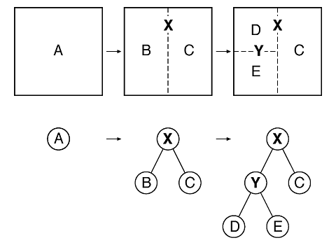
or the ASCII art version:
+-----------+      +-----+-----+      +-----+-----+
|           |      |     |     |      |     |     |
|           |      |     |     |      |  d  |     |
|           |      |     |     |      |     |     |
|     a     |  ->  |  b  X  c  |  ->  +--Y--+  c  |  -> ...
|           |      |     |     |      |     |     |
|           |      |     |     |      |  e  |     |
|           |      |     |     |      |     |     |
+-----------+      +-----+-----+      +-----+-----+
      a                  X                  X           ...
                       -/ \+              -/ \+
                       /   \              /   \
                      b     c            Y     c
                                       -/ \+
                                       /   \
                                      d     e
Other space partitioning structures
BSP trees are closely related to Quadtrees and Octrees. Quadtrees and Octrees are space partitioning trees which recursively divide subspaces into four and eight new subspaces, respectively. A BSP Tree can be used to simulate both of these structures.
--
Last Update: 09/20/101 11:07:07
Overview
Given a set of polygons in three dimensional space, we want to build a BSP tree which contains all of the polygons. For now, we will ignore the question of how the resulting tree is going to be used.
The algorithm to build a BSP tree is very simple:
- Select a partition plane.
- Partition the set of polygons with the plane.
- Recurse with each of the two new sets.
Choosing the partition plane
The choice of partition plane depends on how the tree will be used, and what sort of efficiency criteria you have for the construction. For some purposes, it is appropriate to choose the partition plane from the input set of polygons (called an autopartition). Other applications may benefit more from axis aligned orthogonal partitions.
In any case, you want to evaluate how your choice will affect the results. It is desirable to have a balanced tree, where each leaf contains roughly the same number of polygons. However, there is some cost in achieving this. If a polygon happens to span the partition plane, it will be split into two or more pieces. A poor choice of the partition plane can result in many such splits, and a marked increase in the number of polygons. Usually there will be some trade off between a well balanced tree and a large number of splits.
Partitioning polygons
Partitioning a set of polygons with a plane is done by classifying each member of the set with respect to the plane. If a polygon lies entirely to one side or the other of the plane, then it is not modified, and is added to the partition set for the side that it is on. If a polygon spans the plane, it is split into two or more pieces and the resulting parts are added to the sets associated with either side as appropriate.
When to stop
The decision to terminate tree construction is, again, a matter of the specific application. Some methods terminate when the number of polygons in a leaf node is below a maximum value. Other methods continue until every polygon is placed in an internal node. Another criteria is a maximum tree depth.
Pseudo C++ code example
Here is an example of how you might code a BSP tree:
struct	BSP_tree
{
   plane     partition;
   list      polygons;
   BSP_tree  *front,
             *back;
};
This structure definition will be used for all subsequent example code. It stores pointers to its children, the partitioning plane for the node, and a list of polygons coincident with the partition plane. For this example, there will always be at least one polygon in the coincident list: the polygon used to determine the partition plane. A constructor method for this structure should initialize the child pointers to NULL.
void	Build_BSP_Tree (BSP_tree *tree, list polygons)
{
   polygon   *root = polygons.Get_From_List ();
   tree->partition = root->Get_Plane ();
   tree->polygons.Add_To_List (root);
   list      front_list,
             back_list;
   polygon   *poly;
   while ((poly = polygons.Get_From_List ()) != 0)
   {
      int   result = tree->partition.Classify_Polygon (poly);
      switch (result)
      {
         case COINCIDENT:
            tree->polygons.Add_To_List (poly);
            break;
         case IN_BACK_OF:
            back_list.Add_To_List (poly);
            break;
         case IN_FRONT_OF:
            front_list.Add_To_List (poly);
            break;
         case SPANNING:
            polygon   *front_piece, *back_piece;
            Split_Polygon (poly, tree->partition, front_piece, back_piece);
            back_list.Add_To_List (back_piece);
            front_list.Add_To_List (front_piece);
            break;
      }
   }
   if ( ! front_list.Is_Empty_List ())
   {
      tree->front = new BSP_tree;
      Build_BSP_Tree (tree->front, front_list);
   }
   if ( ! back_list.Is_Empty_List ())
   {
      tree->back = new BSP_tree;
      Build_BSP_Tree (tree->back, back_list);
   }
}
This routine recursively constructs a BSP tree using the above definition. It takes the first polygon from the input list and uses it to partition the remainder of the set. The routine then calls itself recursively with each of the two partitions. This implementation assumes that all of the input polygons are convex.
One obvious improvement to this example is to choose the partitioning plane more intelligently. This issue is addressed separately in the section, "How can you make a BSP Tree more efficient?".
--
Last Update: 09/06/101 14:50:29
Overview
Partitioning a polygon with a plane is a matter of determining which side of the plane the polygon is on. This is referred to as a front/back test, and is performed by testing each point in the polygon against the plane. If all of the points lie to one side of the plane, then the entire polygon is on that side and does not need to be split. If some points lie on both sides of the plane, then the polygon is split into two or more pieces.
The basic algorithm is to loop across all the edges of the polygon and find those for which one vertex is on each side of the partition plane. The intersection points of these edges and the plane are computed, and those points are used as new vertices for the resulting pieces.
Implementation notes
Classifying a point with respect to a plane is done by passing the (x, y, z) values of the point into the plane equation, Ax + By + Cz + D = 0. The result of this operation is the distance from the plane to the point along the plane's normal vector. It will be positive if the point is on the side of the plane pointed to by the normal vector, negative otherwise. If the result is 0, the point is on the plane.
For those not familiar with the plane equation, The values A, B, and C are the coordinate values of the normal vector. D can be calculated by substituting a point known to be on the plane for x, y, and z.
Convex polygons are generally easier to deal with in BSP tree construction than concave ones, because splitting them with a plane always results in exactly two convex pieces. Furthermore, the algorithm for splitting convex polygons is straightforward and robust. Splitting of concave polygons, especially self intersecting ones, is a significant problem in its own right.
Pseudo C++ code example
Here is a very basic function to split a convex polygon with a plane:
void Split_Polygon (polygon *poly, plane *part, polygon *&front, polygon *&back)
{
   int   count = poly->NumVertices (),
         out_c = 0, in_c = 0;
   point ptA, ptB,
         outpts[MAXPTS],
         inpts[MAXPTS];
   real	sideA, sideB;
   ptA = poly->Vertex (count - 1);
   sideA = part->Classify_Point (ptA);
   for (short i = -1; ++i < count;)
   {
      ptB = poly->Vertex (i);
      sideB = part->Classify_Point (ptB);
      if (sideB > 0)
      {
         if (sideA < 0)
         {
            // compute the intersection point of the line
            // from point A to point B with the partition
            // plane. This is a simple ray-plane intersection.
            vector v = ptB - ptA;
            real   sect = - part->Classify_Point (ptA) / (part->Normal () | v);
            outpts[out_c++] = inpts[in_c++] = ptA + (v * sect);
         }
         outpts[out_c++] = ptB;
      }
      else if (sideB < 0)
      {
         if (sideA > 0)
         {
            // compute the intersection point of the line
            // from point A to point B with the partition
            // plane. This is a simple ray-plane intersection.
            vector v = ptB - ptA;
            real   sect = - part->Classify_Point (ptA) / (part->Normal () | v);
            outpts[out_c++] = inpts[in_c++] = ptA + (v * sect);
         }
         inpts[in_c++] = ptB;
      }
      else
         outpts[out_c++] = inpts[in_c++] = ptB;
      ptA = ptB;
      sideA = sideB;
   }
   front = new polygon (outpts, out_c);
   back = new polygon (inpts, in_c);
}
A simple extension to this code that is good for BSP trees is to combine its functionality with the routine to classify a polygon with respect to a plane.
Note that this code is not robust, since numerical stability may cause errors in the classification of a point. The standard solution is to make the plane "thick" by use of an epsilon value.
--
Last Update: 09/06/101 14:50:29
Overview
Probably the most common application of BSP trees is hidden surface removal in three dimensions. BSP trees provide an elegant, efficient method for sorting polygons via a depth first tree walk. This fact can be exploited in a back to front "painter's algorithm" approach to the visible surface problem, or a front to back scanline approach.
BSP trees are well suited to interactive display of static (not moving) geometry because the tree can be constructed as a preprocess. Then the display from any arbitrary viewpoint can be done in linear time. Adding dynamic (moving) objects to the scene is discussed in another section of this document.
Painter's algorithm
The idea behind the painter's algorithm is to draw polygons far away from the eye first, followed by drawing those that are close to the eye. Hidden surfaces will be written over in the image as the surfaces that obscure them are drawn. One condition for a successful painter's algorithm is that there be a single plane which separates any two objects. This means that it might be necessary to split polygons in certain configurations. For example, this case can not be drawn correctly with a painter's algorithm:
                          +------+
                          |      |
          +---------------|      |--+
          |               |      |  |
          |               |      |  |
          |               |      |  |
          |      +--------|      |--+
          |      |        |      |
       +--|      |--------+      |
       |  |      |               |
       |  |      |               |
       |  |      |               |
       +--|      |---------------+
          |      |
          +------+
One reason that BSP trees are so elegant for the painter's algorithm is that the splitting of difficult polygons is an automatic part of tree construction. Note that only one of these two polygons needs to be split in order to resolve the problem.To draw the contents of the tree, perform a back to front tree traversal. Begin at the root node and classify the eye point with respect to its partition plane. Draw the subtree at the far child from the eye, then draw the polygons in this node, then draw the near subtree. Repeat this procedure recursively for each subtree.
Scanline hidden surface removal
It is just as easy to traverse the BSP tree in front to back order as it is for back to front. We can use this to our advantage in a scanline method method by using a write mask which will prevent pixels from being written more than once. This will represent significant speedups if a complex lighting model is evaluated for each pixel, because the painter's algorithm will blindly evaluate the same pixel many times.
The trick to making a scanline approach successful is to have an efficient method for masking pixels. One way to do this is to maintain a list of pixel spans which have not yet been written to for each scan line. For each polygon scan converted, only pixels in the available spans are written, and the spans are updated accordingly.
The scan line spans can be represented as binary trees, which are just one dimensional BSP trees. This technique can be expanded to a two dimensional screen coverage algorithm using a two dimensional BSP tree to represent the masked regions. Any convex partitioning scheme, such as a quadtree, can be used with similar effect.
Implementation notes
When building a BSP tree specifically for hidden surface removal, the partition planes are usually chosen from the input polygon set. However, any arbitrary plane can be used if there are no intersecting or concave polygons, as in the example above.
Pseudo C++ code example
Using the BSP_tree structure defined in the section, "How do you build a BSP Tree?", here is a simple example of a back to front tree traversal:
void	Draw_BSP_Tree (BSP_tree *tree, point eye)
{
   real   result = tree->partition.Classify_Point (eye);
   if (result > 0)
   {
      Draw_BSP_Tree (tree->back, eye);
      tree->polygons.Draw_Polygon_List ();
      Draw_BSP_Tree (tree->front, eye);
   }
   else if (result < 0)
   {
      Draw_BSP_Tree (tree->front, eye);
      tree->polygons.Draw_Polygon_List ();
      Draw_BSP_Tree (tree->back, eye);
   }
   else // result is 0
   {
      // the eye point is on the partition plane...
      Draw_BSP_Tree (tree->front, eye);
      Draw_BSP_Tree (tree->back, eye);
   }
}
If the eye point is classified as being on the partition plane, the drawing order is unclear. This is not a problem if the Draw_Polygon_List routine is smart enough to not draw polygons that are not within the viewing frustum. The coincident polygon list does not need to be drawn in this case, because those polygons will not be visible to the user.It is possible to substantially improve the quality of this example by including the viewing direction vector in the computation. You can determine that entire subtrees are behind the viewer by comparing the view vector to the partition plane normal vector. This test can also make a better decision about tree drawing when the eye point lies on the partition plane. It is worth noting that this improvement resembles the method for tracing a ray through a BSP tree, which is discussed in another section of this document.
Front to back tree traversal is accomplished in exactly the same manner, except that the recursive calls to Draw_BSP_Tree occur in reverse order.
--
Last Update: 09/06/101 14:50:29
Overview
Analytic visibility is a term which describes the list of surfaces visible from a single point in a scene. Analytic visibility is important to the architectural community because it may be necessary to obtain a visible lines only view of a building for output to a pen plotter. It is also important to the global illumination community because it makes it possible to accurately compute the form factor from a differential area to a patch. Analytic visibility is also used in a preprocessing step to speed up walkthrough renderings for large models.
BSP trees can be used to compute visible fragments of polygons in a scene in at least two different ways. Both methods involve the use of a bsp tree for front to back traversal, and a second tree which describes the visible space in the viewing volume.
Screen partitioning
This method uses a two dimensional BSP tree to partition the viewing plane into regions which have and have not been covered by previously rendered polygons. Whenever a polygon is rendered, it is inserted into the screen tree and clipped to the currently visible region. In the process, the visible region of the polygon is removed from the visible region of the screen.
Beam tree
This method clips each polygon drawn to a beam tree which defines the viewable area. The beam tree originates as a description of the viewing frustum, and is in fact a special kind of BSP tree. When a new polygon is rendered, it is first passed through the beam tree to obtain the visible fragments in a manner very similar to the union operation for boolean modelling. Each fragment is then used to describe a new beam consisting of a series of planes through the eye point and each edge of the fragment. These planes become the hyperplanes used for defining new partitions in the beam tree.
First DRAFT.
--
Last Update: 09/06/101 14:50:28
Overview
Ray tracing with a BSP tree is very similar to hidden surface removal with a BSP tree. The algorithm is a simple forward tree walk, with a few additions that apply to ray casting. See Jim Arvo's voxel walking algorithm for ray tracing excerpted from the Ray Tracing News.
Implementation notes
Probably the biggest difference between ray tracing and other applications of BSP trees is that ray tracing does not require splitting of primitives to obtain correct results. This means that the hyperplanes can, and should, be chosen strictly for tree balance.
A large improvement can be made over the voxel walking algorithm for recursive ray tracing by using the parent node of the ray origin as a hint.
Because ray tracing is a spatial classification problem, balancing is the key to performance. Most spatial partitioning schemes for accellerating ray tracing use a criteria called "occupancy", which refers to the number of primitives residing in each partition. A BSP tree which has approximately the same occupancy for all partitions is balanced.
Balancing is discussed elsewhere in this document.
MORE TO COME
--
Last Update: 09/20/101 11:05:05
Overview
There are two major classes of solid modeling methods with BSP trees. For both methods, it is useful to introduce the notion of an in/out test.
An in/out test is a different way of talking about the front/back test we have been using to classify points with respect to planes. The necessity for this shift in thought is evident when considering polytopes instead of just polygons. A point can not be merely in front or back of a polytope, but inside or outside. Somewhat formally, a point is inside of a convex polytope if it is inside of, or in back of, each hyperplane which composes the polytope, otherwise it is outside.
Incremental construction
Incremental construction of a BSP Tree is the process of inserting convex polytopes into the tree one by one. Each polytope has to be processed according to the operation desired.
It is useful to examine the construction process in two dimensions. Consider the following figure:
A               B
 +-------------+
 |             |
 |             |
 |      E      |        F
 |       +-----+-------+
 |       |     |       |
 |       |     |       |
 |       |     |       |
 +-------+-----+       |
D        |      C      |
         |             |
         |             |
         +-------------+
        H               G
Two polygons, ABCD, and EFGH, are to be inserted into the tree. We wish to find the union of these two polygons. Start by inserting polygon ABCD into the tree, choosing the splitting hyperplanes to be coincident with the edges. The tree looks like this after insertion of ABCD:
                AB
              -/  \+
              /    \
             /      *
            BC
          -/  \+
          /    \
         /      *
        CD
      -/  \+
      /    \
     /      *
    DA
  -/  \+
  /    \
 *      *
Now, polygon EFGH is inserted into the tree, one edge at a time. The result looks like this:
A               B
 +-------------+
 |             |
 |             |
 |      E      |J       F
 |       +-----+-------+
 |       |     |       |
 |       |     |       |
 |       |     |       |
 +-------+-----+       |
D        |L    :C      |
         |     :       |
         |     :       |
         +-----+-------+
        H      K        G
                        AB
                      -/  \+
                      /    \
                     /      *
                    BC
                  -/  \+
                  /    \
                 /      \
                CD       \
              -/  \+      \
              /    \       \
             /      \       \
            DA       \       \
          -/  \+      \       \
          /    \       \       \
         /      *       \       \
        EJ              KH       \
      -/  \+          -/  \+      \
      /    \          /    \       \
     /      *        /      *       \
    LE              HL              JF
  -/  \+          -/  \+          -/  \+
  /    \          /    \          /    \
 *      *        *      *        FG     *
                               -/  \+
                               /    \
                              /      *
                             GK
                           -/  \+
                           /    \
                          *      *
Notice that when we insert EFGH, we split edges EF and HE along the edges of ABCD. this has the effect of dividing these segments into pieces which are inside ABCD, and outside ABCD. Segments EJ and LE will not be part of the boundary of the union. We could have saved our selves some work by not inserting them into the tree at all. For a union operation, you can always throw away segments that land in inside nodes. You must be careful about this though. What I mean is that any segments which land in inside nodes of the pre-existing tree, not the tree as it is being constructed. EJ and LE landed in an inside node of the tree for polygon ABCD, and so can be discarded.Our tree now looks like this:
A               B
 +-------------+
 |             |
 |             |
 |             |J       F
 |             +-------+
 |             |       |
 |             |       |
 |             |       |
 +-------+-----+       |
D        |L    :C      |
         |     :       |
         |     :       |
         +-----+-------+
        H      K        G
                        AB
                      -/  \+
                      /    \
                     /      *
                    BC
                  -/  \+
                  /    \
                 /      \
                CD       \
              -/  \+      \
              /    \       \
             /      \       \
            DA       \       \
          -/  \+      \       \
          /    \       \       \
         *      *       \       \
                        KH       \
                      -/  \+      \
                      /    \       \
                     /      *       \
                    HL              JF
                  -/  \+          -/  \+
                  /    \          /    \
                 *      *        FG     *
                               -/  \+
                               /    \
                              /      *
                             GK
                           -/  \+
                           /    \
                          *      *
Now, we would like some way to eliminate the segments JC and CL, so that we will be left with the boundary segments of the union. Examine the segment BC in the tree. What we would like to do is split BC with the hyperplane JF. Conveniently, we can do this by pushing the BC segment through the node for JF. The resulting segments can be classified with the rest of the JF subtree. Notice that the segment BJ lands in an out node, and that JC lands in an in node. Remembering that we can discard interior nodes, we can eliminate JC. The segment BJ replaces BC in the original tree. This process is repeated for segment CD, yielding the segments CL and LD. CL is discarded as landing in an interior node, and LD replaces CD in the original tree. The result looks like this:
A               B
 +-------------+
 |             |
 |             |
 |             |J       F
 |             +-------+
 |                     |
 |                     |
 |        L            |
 +-------+             |
D        |             |
         |             |
         |             |
         +-----+-------+
        H      K        G
                        AB
                      -/  \+
                      /    \
                     /      *
                    BJ
                  -/  \+
                  /    \
                 /      \
                LD       \
              -/  \+      \
              /    \       \
             /      \       \
            DA       \       \
          -/  \+      \       \
          /    \       \       \
         *      *       \       \
                        KH       \
                      -/  \+      \
                      /    \       \
                     /      *       \
                    HL              JF
                  -/  \+          -/  \+
                  /    \          /    \
                 *      *        FG     *
                               -/  \+
                               /    \
                              /      *
                             GK
                           -/  \+
                           /    \
                          *      *
As you can see, the result is the union of the polygons ABCD and EFGH.To perform other boolean operations, the process is similar. For intersection, you discard segments which land in exterior nodes instead of internal ones. The difference operation is special. It requires that you invert the polytope before insertion. For simple objects, this can be achieved by scaling with a factor of -1. The insertion process is then conducted as an intersection operation, where segments landing in external nodes are discarded.
Tree merging
--
Last Update: 09/06/101 14:50:28
Overview
Detecting whether or not a point moving along a line intersects some object in space is essentially a ray tracing problem. Detecting whether or not two complex objects intersect is something of a tree merging problem.
Typically, motion is computed in a series of Euler steps. This just means that the motion is computed at discrete time intervals using some description of the speed of motion. For any given point P moving from point A with a velocity V, it's location can be computed at time T as P = A + (T * V).
Consider the case where T = 1, and we are computing the motion in one second steps. To find out if the point P has collided with any part of the scene, we will first compute the endpoints of the motion for this time step. P1 = A + V, and P2 = A + (2 * V). These two endpoints will be classified with respect to the BSP tree. If P1 is outside of all objects, and P2 is inside some object, then an intersection has clearly occurred. However, if P2 is also outside, we still have to check for a collision in between.
Two approaches are possible. The first is commonly used in applications like games, where speed is critical, and accuracy is not. This approach is to recursively divide the motion segment in half, and check the midpoint for containment by some object. Typically, it is good enough to say that an intersection occurred, and not be very accurate about where it occurred.
The second approach, which is more accurate, but also more time consuming, is to treat the motion segment as a ray, and intersect the ray with the BSP Tree. This also has the advantage that the motion resulting from the impact can be computed more accurately.
--
Last Update: 09/06/101 14:50:28
Overview
So far the discussion of BSP tree structures has been limited to handling objects that don't move. However, because the hidden surface removal algorithm is so simple and efficient, it would be nice if it could be used with dynamic scenes too. Faster animation is the goal for many applications, most especially games.
The BSP tree hidden surface removal algorithm can easily be extended to allow for dynamic objects. For each frame, start with a BSP tree containing all the static objects in the scene, and reinsert the dynamic objects. While this is straightforward to implement, it can involve substantial computation.
If a dynamic object is separated from each static object by a plane, the dynamic object can be represented as a single point regardless of its complexity. This can dramatically reduce the computation per frame because only one node per dynamic object is inserted into the BSP tree. Compare that to one node for every polygon in the object, and the reason for the savings is obvious. During tree traversal, each point is expanded into the original object.
Implementation notes
Inserting a point into the BSP tree is very cheap, because there is only one front/back test at each node. Points are never split, which explains the requirement of separation by a plane. The dynamic object will always be drawn completely in front of the static objects behind it.
A dynamic object inserted into the tree as a point can become a child of either a static or dynamic node. If the parent is a static node, perform a front/back test and insert the new node appropriately. If it is a dynamic node, a different front/back test is necessary, because a point doesn't partition three dimesnional space. The correct front/back test is to simply compare distances to the eye. Once computed, this distance can be cached at the node until the frame is drawn.
An alternative when inserting a dynamic node is to construct a plane whose normal is the vector from the point to the eye. This plane is used in front/back tests just like the partition plane in a static node. The plane should be computed lazily and it is not necessary to normalize the vector.
Cleanup at the end of each frame is easy. A static node can never be a child of a dynamic node, since all dynamic nodes are inserted after the static tree is completed. This implies that all subtrees of dynamic nodes can be removed at the same time as the dynamic parent node.
Caveats
Recent discussion on comp.graphics.algorithms has demonstrated some weaknesses with this approach. In particular, an object modelled as a point may not be rendered in the correct order if the actual object spans a partitioning plane.
Advanced methods
Tree merging, "ghosts", real dynamic trees... MORE TO COME
--
Last Update: 09/06/101 14:50:29
Overview
--
Last Update: 09/06/101 14:50:29
Overview
--
Last Update: 09/06/101 14:50:29
Overview
BSP trees are useful for building an "exact cell decomposition". A cell is any region which is used
as a node in a planning graph. An exact cell decomposition is one in which every cell is entirely
occupied, or entirely empty. The alternative is an "approximate cell decomposition", in which cells
may also be partially occupied. A regular grid on a complex scene is an example of an "approximate
cell decomposition".
Example
Consider a game which uses randomly oriented blocks for obstacles in an enclosed arena. For purposes
of path planning, we are interested in the decomposition of the ground plane. We can get this by
building a BSP tree containing all of the blocks, and pass a polygon which represents the ground
into the tree. The splitting routine should be modified to maintain connectivity information when
splitting polygons. Using a technique similar to boolean modelling, we can reduce the tree to
contain only those polygons which are the regions of the ground plane not contained inside any
obstacles.
Now, a planning graph can be built, using some point inside of each polygon, and connecting to a point inside of each of its neighbors. Note that the selection of the point location has implications for the length of resulting paths. Planning begins by identifying the cell which contains the start point, and the cell which contains the end point. Then a standard A* style search can be used on the planning graph to find the set of polygons that must be crossed to get to the end point from the start point.
Implementation Notes
A simple optimization can help yield a straight path where on is important. When planning
through a given region, keep track of where you are coming from and where you are going to. By
treating the edges of the region as portals, and allowing your entry and exit points to slide along
the portals, you can insure a minimum length path through each node.
FIRST DRAFT
--
Last Update: 09/06/101 14:50:29
Overview
--
Last Update: 09/06/101 14:50:29
Overview
--
Last Update: 09/06/101 14:50:29
Space complexity
For the problem of hidden surface removal, consider a set of n parallel polygons, and the set of m partitioning planes, all of
which are perpendicular to the polgyons. This has the effect of splitting every polygon with every
partition. The number of polygons resulting from this partitioning scheme is n + (n *
m). If the partitioning planes are selected from the candidate polygon set (an
autopartition), then m = n, and the expression reduces to n^2 + n. Thus the worst case spatial complexity of a BSP
tree constructed using an autopartition is O(n^2).
It will be extremely difficult to construct a case which satisfies this formula. The "expected" case, repeatedly expressed by Naylor, is O(n).
Time complexity
The time complexity of rendering from a BSP built using an autopartition is the same as the spatial
complexity, that is a worst case of O(n^2), and an "expected" case of O(n).
--
Last Update: 09/06/101 14:50:28
Bounding volumes
Bounding spheres are simple to implement, take only a single plane comparison, using the center of the sphere.
Optimal trees
Construction of an optimal tree is an NP-complete problem. The problem is one of splitting versus tree balancing. These are mutually exclusive requirements. You should choose your strategy for building a good tree based on how you intend to use the tree.
Minimizing splitting
An obvious problem with BSP trees is that polygons get split during the construction phase, which results in a larger number of polygons. Larger numbers of polygons translate into larger storage requirements and longer tree traversal times. This is undesirable in all applications of BSP trees, so some scheme for minimizing splitting will improve tree performance.
Bear in mind that minimization of splitting requires pre-existing knowledge about all of the polygons that will be inserted into the tree. This knowledge may not exist for interactive uses such as solid modelling.
Tree balancing
Tree balancing is important for uses which perform spatial classification of points, lines, and surfaces. This includes ray tracing and solid modelling. Tree balancing is important for these applications because the time complexity for classification is based on the depth of the tree. Unbalanced trees have deeper subtrees, and therefore have a worse worst case.
For the hidden surface problem, balancing doesn't significantly affect runtime. This is because the expected time complexity for tree traversal is linear on the number of polygons in the tree, rather than the depth of the tree.
Balancing vs. splitting
If balancing is an important concern for your application, it will be necessary to trade off some balance for reduced splitting. If you are choosing your hyperplanes from the polygon candidates, then one way to optimize these two factors is to randomly select a small number of candidates. These new candidates are tested against the full list for splitting and balancing efficiency. A linear combination of the two efficiencies is used to rank the candidates, and the best one is chosen.
Reference Counting
Other Optimizations
--
Last Update: 09/06/101 14:50:28
Overview
A BSP tree resembles a standard binary tree structure in many ways. Using the tree for a painter's algorithm or for ray tracing is a "depth first" traversal of the tree structure. Depth first traversal is traditionally presented as a recursive operation, but can also be performed using an explicit stack.
Implementation Notes
Depth first traversal is a means of enumerating all of the leaves of a tree in sorted order. This is accomplished by visiting each child of each node in a recursive manner as follows:
void    Enumerate (BSP_tree *tree)
{
   if (tree->front)
      Enumerate (tree->front);
   if (tree->back)
      Enumerate (tree->back);
}
To eliminate the recursion, you have to explicitly model the recursion using a stack. Using a stack of pointers to BSP_tree, you can perform the enumeration like this:
void    Enumerate (BSP_tree *tree)
{
   Stack  stack;
   while (tree)
   {
      if (tree->back)
         stack.Push (tree->back);
      if (tree->front)
         stack.Push (tree->front);
      tree = stack.Pop ();
   }
}
On some processors, using a stack will be faster than the recursive method. This is especially true if the recursive routine has a lot of local variables. However, the recursive approach is usually easier to understand and debug, as well as requiring less code.
--
Last Update: 09/06/101 14:50:28
Overview
Neophyte: How did the BSP-Tree come to be?
Sage: Long ago in a small village in Nepal, a minor godling gave a special nut to the priests at an out of the way temple. With the nut, was a prophecy: When a group of three gurus, two with red hair, and the other who was not what he seemed, came to the temple on pilgrimage, if the nut was given unto them, and they nurtured it together, it would produce a tree of great benefit to mankind. Many years later, ...
N: no! No! NO! The TRUE story.
S: OK.
Long ago (by computer industry standards) in a rapidly growing sunbelt city in Texas, a serendipitous convergence of unusual talents and personalities occurred. A brief burst of graphics wonderments appeared, and the convergence diverged under its own explosive production, leading to further graphics developments in several new locations. One of the wonderous paths followed ...
N: ...No! The facts!
S: Huh? Oh you want FACTS. Boring stuff?
Henry Fuchs started teaching at an essentially brand new campus, the University of Texas at Dallas, in January 1975. He returned to Utah to complete his PhD the following summer. He returned to Dallas and taught for the 1975-76, 1976-77 and 1977-78 academic years, before being lured away to UNC-Chapel Hill.
Zvi Kedem joined this faculty in the fall of 1975. He was (and still is I suppose) a "theory person," but a special theory person. He is good at applying theory to practical problems.
Bruce Naylor had a bachelors degree from the U of Texas (Austin - "the real one"), in philosophy if I recall correctly. He had talked his way into a job at Texas Instruments in Dallas. (Something about philosophy makes you good in logic, which is really the same as computers...!?) He came to UTD to take some computer courses. He was spotted as "good" - probably by Kedem, but I can't swear to it - and convinced to become a full time graduate student.
Graphics, of course, is dazzling and wonderful. Henry was (is) full of energy and enthusiasm. It was natural that he attracted lots of the grad students. Kedem was a perfect complement, providing not only the formal rigor and proofs, but also the impetus to "write this part up" before going on to "the next thing and the next thing and ..." Kedem and Fuchs together (and most of the grad students) also found a new thrust in the CS theory community, called computational geometry, particularly interesting. Henry liked to talk about the Schumacker priority driven visible surface algorithm when the class got to that topic. He seemed to think there was something more to be done in that vein. Naylor being a grad student in search of a topic, looked into it.
The result was two SIGGRAPH papers and Naylor's PhD dissertation, and the launch of BSP-trees into the world. The two papers are
Fuchs, Kedem and Naylor, "Predeterming Visibility Priority in 3-D Scenes" SIGGRAPH '79, pp 175-181. (subtitled "preliminary report")
and
Fuchs, Kedem and Naylor, "On Visible Surface Generation by A Priori Tree Structures" SIGGRAPH '80, pp124-133.
The first paper isn't really BSP-trees, but rather the preliminary work which led to BSP-trees as the solution. The second paper is the "classic" starting point referenced in texts, etc.
Both reference Schumacker, Brand, Gilliland and Sharp, "Study for Applying Computer-Generated Images to Visual Simulation" AFHRL-TR-69-14, US AF Human Resources Lab, 1969
and the description of this algorithm more easily found in
Sutherland, Sproull and Schumacker, "A Characterization of Ten Hidden Surface Algorithms", ACM Computing Surveys, v 6, no 1, pp 1-55.
Naylor finished in 1981 (?) and went to Georgia Tech, and later to
Bell Labs. He has continued to work on related and similar ideas with
a variety of students and collaborators. Others have also taken the
ideas in new directions.
--
Last Update: 09/06/101 14:50:28
BSP tree FAQ companion code
The companion source code to this document is available via FTP at:
Also in this directory is the BSP tree demo application for MacOS and Win95. This demo shows how to use BSP trees for basic Boolean modelling and hidden surface removal, and includes an implementation of Ken Shoemake's ArcBall interface. The MacOS package includes all of the source for the demo application in several Metrowerks CodeWarrior projects. The Win95 package is based on the MacOS package, and includes all the source for the demo in a single Microsoft Visual C++ 4.2 project. An X-Windows port is in progress.
Information about the ArcBall controller can be found in Graphics Gems IV (see below). The original paper and demo application for 68k based Apple Macintosh computers is available via WWW or FTP at:
- http://www.cis.upenn.edu/ftpbin/ftphtml.pl?/pub/graphics/arcball
- ftp://ftp.cis.upenn.edu/pub/graphics/arcball/
Graphics Gems
The Graphics Gems archive is available via FTP at:
- ftp://ftp.princeton.edu/pub/Graphics/GraphicsGems/
- ftp://ftp-graphics.stanford.edu/pub/Graphics/GraphicsGems/
It is an invaluable resource for all things graphical. In particular, there are some BSP tree references worth looking over.
Peter Shirley and Kelvin Sung have C sample code for ray tracing with BSP trees in Graphics Gems III
Norman Chin has provided a wonderful resource for BSP trees in Graphics Gems V. He provides C sample code for a wide variety of uses.
Other BSP tree resources
The Ray Tracing News is available at:
It has many good articles which involve the use of BSP trees or compares them to other data structures for ray tracing efficiency. It's definitely worth a look.
The DejaNews research service is a search engine for newsgroup postings. Conduct a search on "BSP tree" to read over recent, as well as old, discussions about BSP trees. DejaNews is available at:
Pat Fleckenstein and Rob Reay have put together a FAQ on 3D graphics, which includes a blurb on BSP trees, and an FTP site with some sample code:
Dr. Dobbs Journal has an article in their July '95 issue about BSP trees, By Nathan Dwyer. It describes the construction of BSP trees for visible surface processing, how to split polygons with planes, and how to dump the tree to a file. There is C++ source code to accompany the article.
Michael Abrash's columns in the DDJ Sourcebooks are an excellent introduction to the concept of BSP trees, and the practical details of implementing them for games like Doom and Quake. The source code for these articles is distributed over several sites.
Ekkehard Beier has made available a generic 3D graphics kernel intended to assist development of graphics application interfaces. One of the classes in the library is a BSP tree, and full source is provided. The focus seems to be on ray tracing, with the code being based on Jim Arvo's Linear Time Voxel Walking article in the ray tracing news.
Eddie Edwards wrote a commonly referenced text which describes 2D BSP trees in some detail for use in games like DOOM. It includes a bit of sample code, too.
Mel Slater has made available his C source code for computing shadow volumes based on BSP trees. There is also a paper which compares three shadow volume algorithms. These are available via FTP at:
The SPHIGS distribution that accompanies the famous Foley, et al. Computer Graphics textbook contains a BSP tree implementation and can be obtained at:
John Holmes, Jr. has a paper about BSP trees and boundary representations online. This paper touches on many aspects of BSP trees in a scientific manner, and is available at:
A.T. Campbell III has placed his doctoral dissertation online. This document describes the use of BSP trees for surface meshing in a radiosity algorithm. He has also made available source code in both C and C++ for many BSP tree tasks, including an implementation of tree merging. This is all available on his home page at:
Andrea Marchini and Stefano Tommesani have made available a BSP tree compiler and viewing program as part of the "Purple Haze" project. There is some nice accompanying documentation of the process of BSP tree construction, as well. The web page is at:
Paton Lewis has built an excellent demonstration of BSP trees using Java. If you have had problems visualizing the tree contruction process, you should take a look at this tool. The user draws lines in an interactive construction space, and three other view panes show the split segments, a traditional graph representation of the tree, and a first person perspective view of the line segments as walls. This is how DOOM works. The web page is:
A general graphics programming resources has an article about building BSP trees using axis-aligned partitioning planes. The article calls this structure a bintree, after a 1994 paper by Tamminen. The URL is:
John Whitley has a short tutorial page about BSP trees which covers general details of tree construction and display. It includes psuedo-code for a front to back tree traversal, and an annotated bibliography. The location of this resource is:
Tom Hammersly has put up a web page with his experience in building a BSP tree compiler and viewer. The web page is at:
Id software has made a great deal of source code for games and utilities available, much of which deals extensively with BSP trees. The source code is complete, and easy to understand. The site is at:
General resources for computer graphics programming
If you are interested in game programming, check out the rec.games.programmer.faq: http://www.io.com/~paulhart/game/FAQ/rgp_FAQ.html. You can also look at Paul's game programming page, http://www.io.com/~paulhart/game/.
The computational geometry web page contains lots of information and pointers to related computational geometry tools and algorithms: http://www.cs.duke.edu/~jeffe/compgeom/. Another computational geometry page to look at is http://www.ics.uci.edu:80/~eppstein/geom.html. This page seems to have a more tutorial nature than the first page.
--
Last Update: 09/20/101 11:05:49
A partial listing of textual info on BSP trees.
--
Last Update: 09/20/101 11:06:34