CS 70 - Lecture 38 - Apr 25, 2011 - 10 Evans
Goals for today: Normal or Gaussian Distribution
Central Limit Theorem
Florida election in 2000:
how close is a 537 vote margin out of 5.8M votes,
when 5800 votes may be counted wrong, on average?
Exponential Distribution
The most important probability distribution in many applications is
Def: A random variable X with density function
f(x) = (1/sqrt(2*pi)) * exp(-x^2/2)
is said to have a standard normal distribution with mean 0 and
standard deviation 1.
More generally, a random variable Y with density function
g(x) = (1/(sigma*sqrt(2*pi)) * exp(-(x-mu)^2/(2*sigma^2))
is said to have a standard normal distribution with mean mu and
standard deviation sigma. This is also called a Gaussian distribution.
The plot of f(x) or g(x) is called a "bell shaped curve."
f(x) is centered at its mean 0 (g(x) at mu), and the width
of the main part of the bell is 2 (2*sigma for g(x)).
Def: The cumulative distribution function (cdf) for either X or Y can be written
P(X <= z) = P( Y-mu <= z*sigma)
= (1/sqrt(2*pi))*integral_{-inf}^z exp(-x^2/2) dx
= Normal(z)
As in Chebyshev's inequality, we use the quantity z to measure
the number of standard deviations sigma the random variable is away from
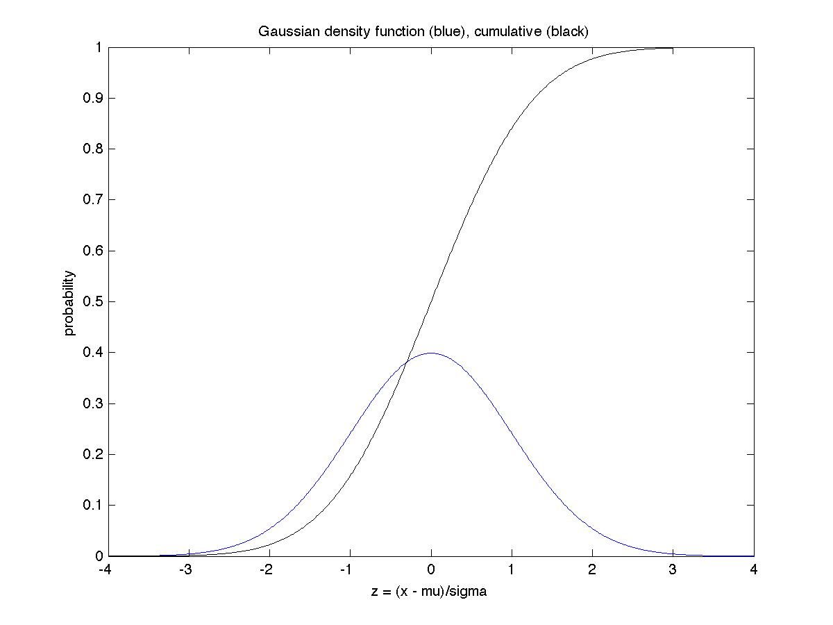
its expectation mu. The plot below shows both f(z) and Normal(z)
for the range -4 to 4. The sides of the bell curve decrease rapidly,
which means that the chance of being far away from the mean is small:
The second column in the table below, Normal(-z), is the probability of
being z standard deviations smaller than the mean, the third column is
the probability of being within z standard deviations of the mean,
and the last column is what Chebyshev's inequality would yield as an
upper bound on Normal(-z); it is clearly much larger than the actual value
Normal(-z).
z Normal(-z) Normal(z)-Normal(-z) Chebyshev / 2
4 3e-5 .99994 1/32 ~ .031
3 .001 .997 1/18 ~ .056
2 .023 .95 1/8 = .125
1 .16 .68 1/2 = .5
We note that there is no simple closed form formula to compute Normal(z).
But it is so important, that historically big tables of its values were
published, and today it is a built-in function in statistical software
packages, and of course there are free webpages that will compute it for you.
The most surprising and important fact about the Gaussian distribution
is how well it approximates so many other distributions, a fact called
the Central Limit Theorem (CLT):
Central Limit Theorem: Let X_i be independent random variables,
continuous or discrete, with expectations mu_i and standard deviations sigma_i.
Let S_n = sum_{i=1 to n} X_i, so that E(S_n) = sum_{i=1 to n} mu_i and
V(S_n) = sum_{i=1 to n} sigma_i^2 = sigma^2(S_n). Then
lim_{n -> inf} P( S_n - E(S_n) <= z*sigma(S_n) ) = Normal(z)
In the special case when the X_i are i.i.d., and so all have
the same expectation mu and standard deviation sigma, we
let A_n = S_n/n and simplify this to
lim_{n -> inf} P( A_n - mu <= z*sigma/sqrt(n) ) = Normal(z)
There are some technical assumptions needed to prove these theorems
(we will not do the proofs, which are hard). It is enough to assume
that all the X_i are bounded, and the sigma_i are also bounded away
from zero (if sigma_i weren't nonzero, X_i wouldn't be "random"!).
The examples below illustrate this theorem in two cases, where the X_i are i.i.d.
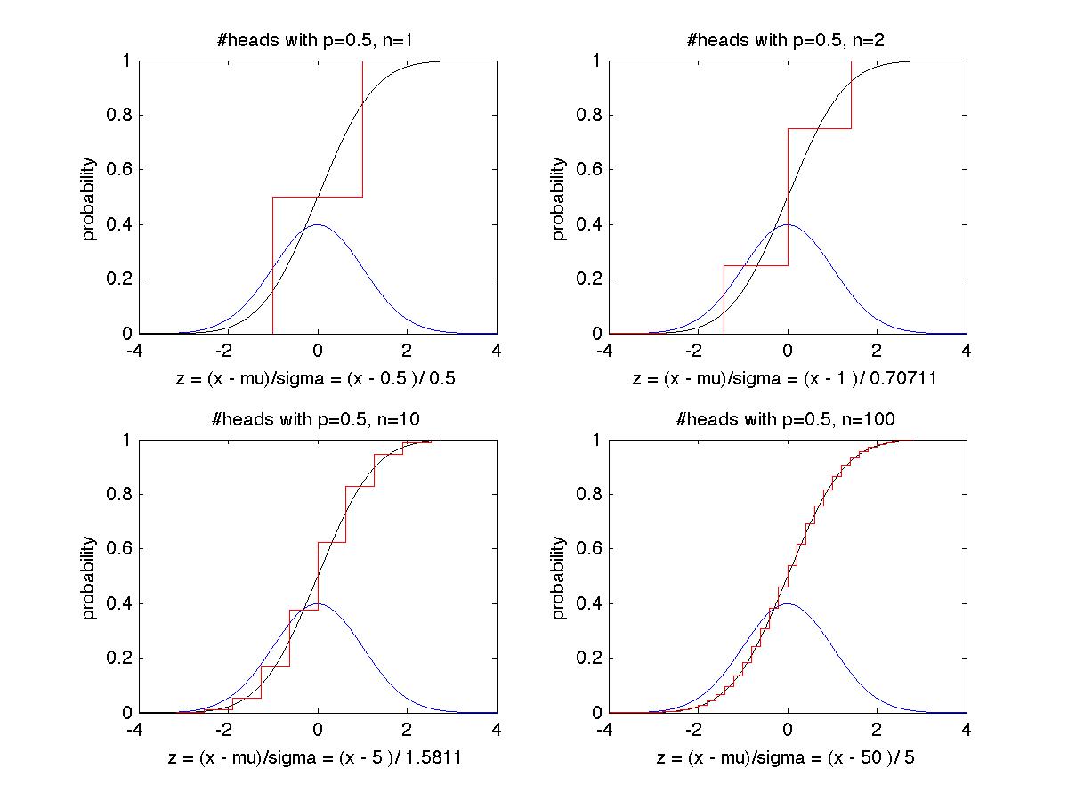
Ex 1: We flip a fair coin n times, where n = 1, 2, 10, and 100 in the four
pictures below, with X_i = 1 if the i-th toss is Heads, and 0 if Tails.
Thus S_n = X_1 + ... + X_n is the number of Heads, and mu = .5 and sigma = .5.
The black and blue curves are the same as in the figure above, and the red curve
C(z) is the true cumulative distribution function for the problem, namely
C(z) = P( (#Heads/n - .5) <= z * .5 / sqrt(n) )
= P( #Heads <= .5 + z * .5/sqrt(n) )
= sum_{i=0 to .5 + z*.5/sqrt(n)} C(n,i)*.5^i*(1-.5)^(n-i)
= sum_{i=0 to .5 + z*.5/sqrt(n)} C(n,i)/2^n
The red curve has steps, because it only changes when .5 + z*.5/sqrt(n)
is an integer from 0 to n. We see that as n increases, the red curve C(z) gets
closer and closer to the black curve Normal(z).
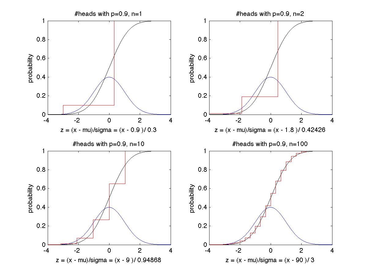
Ex 2: We make the same plots, but with a biased coin where P(H) = .9,
so mu = .9 and sigma = .3. It takes a larger n but eventually
  C(z) = P( (#Heads/n - .9) <= z * .3 / sqrt(n) )
       = sum_{i=0 to .9 + z*.3/sqrt(n)} C(n,i)*.9^i*(.1)^(n-i)
approaches Normal(z) as closely as you like.
The CLT does not require the X_i to be i.i.d. Indeed, one could flip
fair coins, unfair coins, roll dice, ask random people their salaries,
etc., add up all the results to get S_n, and you'd still get a bell curve.
We use general version for our final example:

Ex 3: We consider the 2000 election in Florida. Recall the historical data:
Out of 5,825,043 votes cast, 2,912,790 were counted for Bush,
and 2,912,253 for Gore, a margin of 537 votes.
According to a NY Times article of the time, it is not
unusual for 1 out of 1000 votes to be counted incorrectly; let us model this
by saying that whatever an actual ballot says, it is counted correctly with
probability .999 and incorrectly with probability .001, and that each vote
is counted independently, so it like coin flipping with coin biased to be
"correct" or "Heads" with probability .999, and "incorrect" or "Tails"
with probability .001. Thus, with about 5,825,043 votes,
the expected number of incorrectly counted votes is about 5,825,
or 10 times larger than the winning margin. How can we tell if this
is so close that we need to worry, and count it again more carefully?

To answer this, we will ask the following question: supposing Gore had
actually won, what is the probability that the margin of counted
votes for Bush would be at least 537? If this is tiny, we should feel reassured.
To get an upper bound on this probability, we will assume that Gore
actually won by just one vote to compute this probability (because if he
won by more votes, the chance of miscounting enough votes to get a margin
of 537 for Bush would be even smaller). In other words, we will compute
   P(at least 537 more votes are counted for Bush than Gore |
     there were 2912522 votes for Gore and 2912521 votes for Bush)

To answer this question, we will use the first, more general form of the
Central Limit Theorem:
   Let G_1,...,G_2912522 be i.i.d. random variables representing the
   actual votes for Gore:
     G_i = {+1 with probability .999 (i.e. counted correctly)
           {-1 with probability .001 (i.e. counted incorrectly)
   Similarly, let B_1,...,B_2912521 be i.i.d. random variables representing the
   actual votes for Bush:
     B_i = {-1 with probability .999 (i.e. counted correctly)
           {+1 with probability .001 (i.e. counted incorrectly)
Then S = G_1 + ... + G_2912522 + B_1 + ... + B_2912521
is a sum of independent random variable which counts the margin
of votes counted for Gore (if positive) or Bush (if negative).

The first part of the Central Limit Theorem applies to S, with
   E(G_i) = .998 = -E(B_i)
   V(G_i) = 1-.998^2 ~ .004 = V(B_i)
so E(S) = 2,912,522*.998 - 2,912,521*.998 = .998
   V(S) = 5,825,043*.004 ~ 23277 and sigma(S) ~ 153
The CLT tells us that for n large (and 5,825,043 is large!)
   P( S - E(S) <= z*sigma(S) ) ~ Normal(z)
or
   P( S - .998 <= z*153 ) ~ Normal(z)
or
   P( S <= z*153 + .998 ) ~ Normal(z)
We want to compute P(S <= -537), i.e. that the counted votes
gave Bush a lead of at least 537; solving
   z*153 + .998 = -537
yields z ~ -3.52, so
   P( S <= -537 ) = P(Bush had a margin of at least 537 votes | Gore won)
                  ~ Normal(-3.52)
                  ~ .00021
So we can be reassured...

Exponential Distribution: Recall our discussion of the Poisson distribution:
The physical situations of interest were ones where there were lots of
random physical events, like
  calls to a call center
  accesses to a web service
  ticks on a Geiger counter
caused by a very large number n of entities (callers, web-surfers, radioactive nuclei)
making independent decisions whether or not to call/access a website/decay,
each with very low probability p. We defined lambda = n*p, and showed that it
could be interpreted as the average number of events per time unit
(calls per hour, web accesses per minute, ticks per second).
Then the Poisson distribution told us the probability of getting i events per time unit:
  P(i events per time unit) = exp(-lambda)*lambda^i/i!

The other natural question to ask about such a physical situation is the
distribution of the time between consecutive events, eg between the starts of two calls,
the starts of two web-accesses, or two clicks on the Geiger counter.
This time T is a continuous random variable, with an exponential distribution:
   P(T <= t) = 1 - exp(-lambda*t)
and so a density function
   f(t) = d (1 - exp(-lambda*t))/dt = lambda * exp(-lambda*t)
Another way to see why this intuitively makes sense is that
   P(T > t) = exp(-lambda*t)
gets small very fast, either as t increases, or as the
average number of events-per-time-unit, lambda, increases.
We can compute
   E(T) = integral_0^{infinity} t* lambda*exp(-lambda*t) dt = 1/lambda
This also makes intuitive sense, because if there are lambda events per time unit
on average, the time between events must be 1/lambda.
We can also compute
   V(T) = E(T^2) - (E(T))^2
        = integral_0^{infinity} t^2* lambda*exp(-lambda*t) dt - 1/lambda^2
        = 1/lambda^2