     t = 0
     while t < t_final
         for i = 1 to n          ... n = number_of_particles
             compute f(i) = force on particle i
             move particle i under force f(i) for time dt
         end for
         compute interesting properties of particles
         t = t + dt              ... dt = time increment
     end while
The force on a particle is typically composed of three more basic forces:
     force = external_force
             + nearest_neighbor_force
             + far_field_force
The external forces (e.g. current in the
sharks and fish examples) can be computed
for each particle independently, in an embarrassingly parallel way.
The nearest neighbor forces (e.g. collision forces in the
bouncing balls assignment)
only require interactions with nearest neighbors to compute, and are
still relatively easy to parallelize.
The far field forces like gravity, on the other hand, are more
expensive to compute because the force on each particle depends on all the
other particles. The simplest expression for a far field force f(i)
on particle i is
     for i = 1 to n
         f(i) = sum[ j=1,...,n,  j != i ] f(i,j)
     end for
where f(i,j) is the force on particle i due to particle j. Thus, the cost
seems to rise as O(n2), whereas the external and nearest
neighbor forces
appear to grow like O(n). Even with parallelism, the far field forces will
be much more expensive.
Particle simulations arise in astrophysics and celestial mechanics (gravity is the force), plasma simulation and molecular dynamics (electrostatic attraction or repulsion is the force), and computational fluid dynamics (using the vortex method). The same n-body solutions can also be used in solving elliptic partial differential equations (not just the Poisson equation, which governs gravity and electrostatics) and radiosity calculations in computer graphics (with n mutually illuminating bodies).
All these examples strongly motivate us to find a better n-body algorithm, one that even costs less than O(n2) on a serial machine. Fortunately, it turns out that there are clever divide-and-conquer algorithms which only take O(n log n) or even just O(n) time for this problem.
We give one example of the success of this new algorithm. An astrophysics application, which explored the creation and statistical distribution of galaxies, simulated over 17 million particles (stars) for over 600 time steps. This run took 24 hours on a 512 processor Intel Delta, where each processor sustained 10 Mflops of computational speed, for an aggregate sustained speed of over 5 Gflops. The O(n2) algorithm would have run for well over a year on the same problem. To see interesting pictures of these simulations, click here.
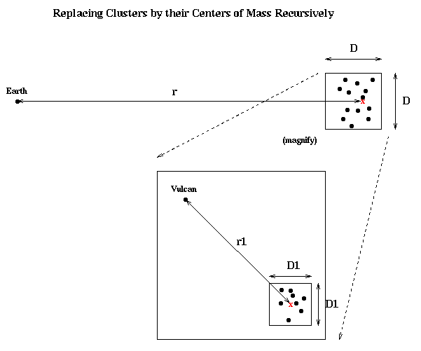
One of those dots of light we might want to include in our sum is, however, not a single star (particle) at all, but rather the Andromeda galaxy, which itself consist of billions of stars. But these appear so close together at this distance that they show up as a single dot to the naked eye. It is tempting -- and correct -- to suspect that it is good enough to treat the Andromeda galaxy as a single point anyway, located at the center of mass of the Andromeda galaxy, and with a mass equal to the total mass of the Andromeda galaxy. This is indicated below, with a red x marking the center of mass. More mathematically, since the ratio
                size of box containing Andromeda
      D/r  = -------------------------------------
             distance of center of mass from Earth
is so small, we can safely and accurately replace the sum over all stars
in Andromeda with one term at their center of mass. (We will justify this
more completely below.)

This idea is hardly new. Indeed, Newton modeled the earth as a single point mass located at its center of mass in order to calculate the attracting force on the falling apple, rather than treating each tiny particle making up the earth separately.
What is new is applying this idea recursively. First, it is clear that from the point of view of an observer in the Andromeda galaxy, our own Milky Way galaxy can also be well approximated by a point mass at our center of mass. But more importantly, within the Andromeda (or Milky Way) galaxy itself, this geometric picture repeats itself as shown below: As long as the ratio D1/r1 is also small, the stars inside the smaller box can be replaced by their center of mass in order to compute the gravitational force on, say, the planet Vulcan. This nesting of boxes within boxes can be repeated recursively.


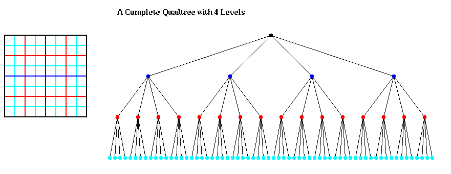
An octtree is similar, but with 8 children per node, corresponding to the 8 subcubes of the larger cube, as illustrated below:

The algorithms we will present begin by constructing a quadtree (or octtree) to store the particles. Thus, the leaves of the tree will contain (or have pointers to) the positions and masses of the particles in the corresponding box.
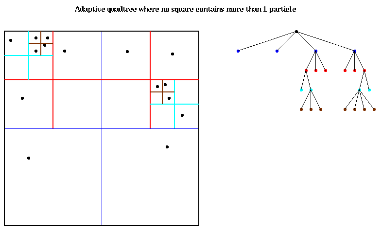
The most interesting problems occur when the particles are not uniformly distributed in their bounding box, so that many of the leaves of a complete quadtree would be empty. In this case, it makes no sense to store these empty parts of the quadtree. Instead, we continue to subdivide squares only when they contain more than 1 particle (or some small number of particles). This leads to the adaptive quadtree shown in the figure below. Note that there are exactly as many leaves as particles. Children are ordered counterclockwise starting at the lower left.

For a much more complicated adaptive quadtree, click here and look at figure 1 on page 2.
Given a list of particle positions, this quadtree can be constructed recursively as follows:
   procedure QuadtreeBuild
     Quadtree = {empty}
       For i = 1 to n          ... loop over all particles
         QuadInsert(i, root)   ... insert particle i in quadtree
       end for
       ... at this point, the quadtree may have some empty
       ... leaves, whose siblings are not empty
       Traverse the tree (via, say, breadth first search),
         eliminating empty leaves

   procedure QuadInsert(i,n)
     ... Try to insert particle i at node n in quadtree
     ... By construction, each leaf will contain either
     ... 1 or 0 particles
     if the subtree rooted at n contains more than 1 particle
        determine which child c of node n particle i lies in
          QuadInsert(i,c)
     else if the subtree rooted at n contains one particle
        ... n is a leaf
        add n's four children to the Quadtree
        move the particle already in n into the child
           in which it lies
        let c be child in which particle i lies
        QuadInsert(i,c)
     else if the subtree rooted at n is empty
        ... n is a leaf
        store particle i in node n
     endif
The complexity of QuadtreeBuild depends on the distribution of the particles
inside the bounding box. The cost of inserting a particle is proportional
to the distance from the root to the leaf in which the particle resides
(measured by the level of the leaf, with the root at level 0).
If the particles are all clustered closely together,
so that they all lie in a single tiny subsquare of the bounding box, then
the complexity can be large because the leaf can be far from the root.
But it cannot be farther than the number of bits b used to represent the
positions of the particles, which we may consider a constant.
If the particles are uniformly distributed, so the leaves of
the quadtree are all on the same level, the complexity of inserting
all the particles will be O(n*log n) = O( n*b ).
(Note that log n <= b, since we can have at most 2b
distinct particles.)
Whether to call this O(n*log n) or O(n) depends on your point of view.
We will return to data structure representations of quadtrees and octtrees when we discuss parallelization. But for now we know enough to discuss the simplest hierarchical n-body algorithm, which is due to Barnes and Hut.
At a high level, here is the Barnes-Hut algorithm:
   1)  Build the Quadtree, using QuadtreeBuild
       as described above.
   2)  For each subsquare in the quadtree,
       compute the center of mass and total mass
       for all the particles it contains.
   3)  For each particle, traverse the tree
       to compute the force on it.
We have already presented the first step of the algorithm in the last subsection. The second step of the algorithm is accomplished by a simple "post order traversal" of the quadtree (post order traversal means the children of a node are processed before the node). Note that the mass and center of mass of each tree node n are stored at n; this is important for the next step of the algorithm.
   ... Compute the center of mass and total mass
   ... for particles in each subsquare
   ( mass, cm ) = Compute_Mass(root)   ... cm = center of mass

   function ( mass, cm ) = Compute_Mass(n)
       ... Compute the mass and center of mass (cm) of
       ... all the particles in the subtree rooted at n
       if n contains 1 particle
            ... the mass and cm of n are identical to
            ... the particle's mass and position
            store ( mass, cm ) at n
            return ( mass, cm )
       else
            for all four children c(i) of n (i=1,2,3,4)
                ( mass(i), cm(i) ) = Compute_Mass(c(i))
            end for
            mass = mass(1) + mass(2) + mass(3) + mass(4)
                 ... the mass of a node is the sum of
                 ... the masses of the children
            cm = (  mass(1)*cm(1) + mass(2)*cm(2)
                  + mass(3)*cm(3) + mass(4)*cm(4)) / mass
                 ... the cm of a node is a weighted sum of
                 ... the cm's of the children
            store ( mass, cm ) at n
            return ( mass, cm )
       end
The cost of this algorithm is proportional to the number of nodes in
the tree, which is no more than O(n), modulo the distribution of
particles (in other words, it could be O(n*log n) or O(n*b) where
b is the number of bits used to represent position).
Finally, we come to the core of the algorithm, computing the force on each particle. We use the idea in the first figure above, namely that if the ratio
    D                      size of box
    -  =  -----------------------------------------------
    r     distance from particle to center of mass of box
is small enough, then we can compute the force due to all the particles
in the box just by using the mass and center of mass of the particles
in the box. We will compare D/r to a user-supplied threshold theta
(usually a little less than 1) to make this decision.
Thus, if D/r < theta, we compute the gravitational force on the particle as follows. Let
Then the gravitational force attracting the particle is approximated by(*) force = G * m * mcm *
xcm - x ycm - y zcm - z
( ---------- , ---------- , ---------- )
r3 r3 r3
where
      r = sqrt(   ( xcm - x )2
                + ( ycm - y )2
                + ( zcm - z )2 )
is the distance from the particle to the center of mass of the particles
in the box.
Here is the algorithm for step 3 of Barnes-Hut:
      ... For each particle, traverse the tree
      ... to compute the force on it.
      For i = 1 to n
          f(i) = TreeForce(i,root)
      end for

      function f = TreeForce(i,n)
          ... Compute gravitational force on particle i
          ... due to all particles in the box at n
          f = 0
          if n contains one particle
              f = force computed using formula (*) above
          else
              r = distance from particle i to
                     center of mass of particles in n
              D = size of box n
              if D/r < theta
                  compute f using formula (*) above
              else
                  for all children c of n
                      f = f + TreeForce(i,c)
                  end for
              end if
          end if
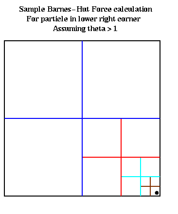
The correctness of the algorithm follows from the fact that the force from each part of the tree is accumulated in f recursively. To understand the complexity, we will show that each call to TreeForce(i,root) has a cost proportional to the depth at which the leaf holding particle i occurs in the tree. To illustrate, consider the figure below, which shows the result of calling TreeForce(i,root) with theta > 1, for the particle i shown in the lower right corner. For each of the unsubdivided squares shown, except the one containing particle i, we have D/r <= 1 < theta. (There are 3 such large blue unsubdivided squares, 3 smaller red squares, 3 yet smaller cyan squares, and 3 smallest brown squares.) Since the test D/r < theta is satisfied for each unsubdivided square, a constant amount of work is done for each unsubdivided square. Since there are at most 3 undivided squares at each level of the tree, the total amount of work for particle i is proportional to the depth at which particle i is stored.

Thus, the total cost of step 3 of the Barnes-Hut algorithm is the sum of the depths in the quadtree at which each particle is stored; as before, this may be bounded either by O(n*log n) or O(n*b).
When theta < 1 -- the usual case -- then it is more complicated to describe which boxes satisfy D/r < theta, but the same O(.) style analysis works.
This completes the discussion of the serial Barnes-Hut algorithm.