Here is the notation we will use in this and subsequent lectures. We consider a weighted, undirected graph G=(N, E, WN, WE) without self edges (i,i) or multiple edges from one node to another. N is the set of nodes, E is the set of edges (i,j) connecting nodes, WN are the node weights, a nonnegative weight for each node, and WE are the edge weights, a nonnegative weight for each edge. When we refer to a graph in this lecture, we will always mean this kind of graph. If WN or WE is omitted from the definition of G, the weight of each node in N and each edge in E is assumed to be 1. We use the notation |N| (or |E|) to mean the number of members of the set N (or E).
We think of a node n in N as representing an independent job to do, and weight Wn as measuring the cost of job n. An edge e=(i,j) in E means that an amount of data We must be transferred from job j to job i to complete the overall task. Partitioning G means dividing N into the union of P disjoint pieces
N = N1 U N2 U ... U NPwhere the nodes (jobs) in Ni are assigned to be done by processor Pi. This partitioning is done subject to the optimality conditions below.
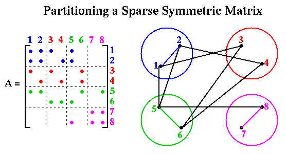
Now we consider in more detail the problem of multiplying a vector x by a sparse symmetric matrix A to get y = A*x. We represent this problem by a graph G with one node i for each xi and yi, and an edge (i,j) for each nonzero Ai,j. We call G the (undirected) graph of the sparse (symmetric) matrix A. To map this problem to a parallel computer, we assume node i stores xi, yi, and Ai,j for all j such that Ai,j is nonzero, and let node i also represent the job of computing yi = sumj Ai,j*xj. We let the weight of node i be the number of floating point multiplications needed to compute yi, i.e. the number of nonzeros in row i of A. We let the weight of each edge (i,j) be one; this represents the cost of sending xj from node j to node i.
Equivalently, we could start with graph G=(N,E), and let the problem be to compute a weighted average yi of a value xi stored at each node i and values xj on neighboring nodes. The reader can confirm that this is equivalent to computing y=A*x with a matrix A whose graph is G, and whose nonzero entries are the weights in the weighted average.
Given a solution of the graph partitioning problem, i.e. an assignment of nodes to processors as in the figure below, the algorithm for computing y=A*x is simply
We present a variety of useful algorithms for solving the graph partitioning problem. For simplicity, we will present most of them with unit weights Wn = 1 and We = 1, although most can be generalized to general weights.
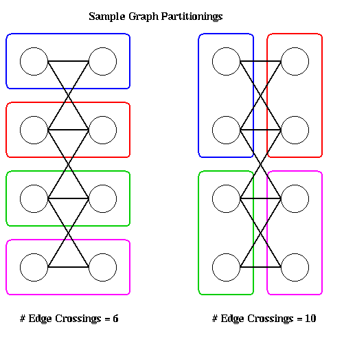
Given n nodes and p processors, there are exponentially many ways to assign n nodes to p processors, some of which more nearly satisfy the optimality conditions than others. To illustrate, the following figure shows two partitions of a graph with 8 nodes onto 4 processors, with 2 nodes per processor. The partitioning on the left has 6 edges crossing processor boundaries and so is superior to the partitioning on the right, with 10 edges crossing processor boundaries. The reader is invited to find another 6-edge-crossing partition, and show that no fewer edge crossings suffice.
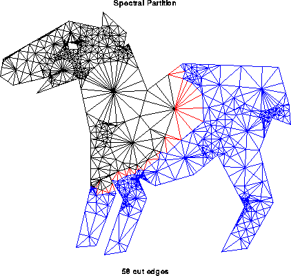
In general, computing the optimal partitioning is an NP-complete problem, which means that the best known algorithms take time which is an exponential function of n=|N| and p, and it is widely believed that no algorithm whose running time is a polynomial function of n=|N| and p exists (see ``Computers and Intractability'', M. Garey and D. Johnson, W. H. Freeman, 1979, for details.) Therefore we need to use heuristics to get approximate solutions for problems where n is large. The picture below illustrates a larger graph partitioning problem; it was generated using the spectral partitioning algorithm as implemented in the graph partitioning software by Gilbert et al, described below. The partition is N = Nblue U Nblack, with red edges connecting nodes in the two partitions.
Almost all the algorithms we discuss are only for graph bisection, i.e. they partition N = N1 U N2. They are intended to be applied recurively, again bisecting N1 and N2, etc., until the partitions are small and numerous enough.
There are two classes of heuristics, depending on the information available about the graph G. In the first case, we have coordinate information with each node, such as (x,y) or (x,y,z) coordinates. This is frequently available if the graph comes from triangulating or otherwise discretizing a physical domain. For example, in the NASA Airfoil, there are (x,y) coordinates associated with each node. (To see the data and be able to manipulate it, start up matlab and type "airfoil". Arrays i and j contains the endpoints of edges -- edge k connects nodes ik and jk -- and arrays x and y contains the node coordinates -- node k is located at (xk , yk) .) Typically, such graphs have the additional property that only nodes which are spatially close together have edges connecting them. We may use this property to develop two efficient geometrical algorithms for graph partitioning.
For graphs with coordinate information, the partitioning heuristics are geometric, in the following sense. Assume first that their are two coordinates x and y, i.e. that the node lie in the plane. Then the algorithms seek either a line or a circle that divide the nodes in half, with (about) half the nodes on one side of the line or circle, and the rest on the other side. All these algorithm work by trying to find a geometric ``middle'' of the nodes (there are several definitions of middle) and then pass a line (or plane) or circle (or sphere) through this middle point. Note that these algorithm completely ignore where the edges are; they implicitly assume that edges connect nearby nodes only. If the graph satisfies some reasonable properties (which often arise in finite element meshes), then one can prove that the best of these algorithms find good partitions (i.e. split the nodes nearly in half while cutting a nearly minimal number of edges).
The second kind of graph we want to partition is coordinate free, i.e. we have no identification of a node with a physical point in space. In addition, edges have no simple interpretation such as representing physical proximity. These kinds of graphs require combinatorial rather than geometric algorithms to partition them (although obviously combinatorial algorithms may also be applied to graphs with coordinate information).
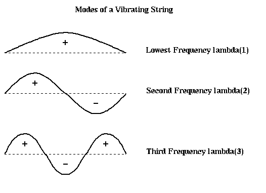
The earliest algorithms used a graph algorithm called breadth first search, which works well for some finite element meshes. The Kernighan-Lin algorithm (the same Kernighan that designed the language C) takes an initial partitioning and iteratively improves it by trying to swap groups of nodes between N1 and N2, greedily picking the group to swap that best minimizes the number of edge crossings at each step. In practice it converges quickly to a (local) optimum if it has a good starting partition. Most recently, the spectral partitioning algorithm was devised, based on the intuition that the second lowest vibrational mode of a vibrating string naturally divides the string in half:
Finally, many of the above algorithms can be accelerated by using a multilevel technique analogous to the multigrid method studied in Lecture 17. The idea is to replace the graph by a coarser graph with many fewer nodes (this was easy to see how to do with rectangular grids in Lecture 17 -- take every other node -- but is a little harder for general graphs), partition the coarser (and so easier) graph, and use the coarse partition as a starting guess for a partition of the original graph. The coarse graph may in turn be partitioned by using the same algorithm recursively: a yet coarser graph is partitioned to get a starting guess, and so on.
Which algorithm is best? As of this writing, Kernighan-Lin combined with the multilevel technique is the fastest available technique, although the geometric methods are also fast and effective on graphs with appropriate properties. The multilevel Kernighan-Lin algorithm is available both in the Chaco and METIS packages described below. After discussing these methods in subsequent sections, we will return to discuss the performance of many of these methods on a set of test problems.
Another package is called Chaco, available from Bruce Hendrickson at Los Alamos National Labs, bahendr@cs.sandia.gov. ("The Chaco User's Guide, Version 1.0", Technical Report SAND93-2339, Sandia National Labs, Albuquerque NM 1993). The Matlab software described above also provides an interface to the algorithms in Chaco, although Chaco must still be obtained directly from Los Alamos. There are more details in the file meshpart.uu.
The package METIS by George Karypis at the University of Minnesota is also available electronically.
Both METIS and Chaco include implementations of multi-level Kernighan-Lin, the currently fastest available algorithm.
Yet another package is JOSTLE, which was written by C. Walshaw, M. Cross, and M. Everett at the University of Greenwich in the UK. It is available free to researchers, but a license agreement is involved. Further information is available here, and the license agreement is here.
The other way to bisect a graph is to find a vertex separator, a subset Ns of N, such that removing Ns and all incident edges from G also results in two disconnected subgraphs G1 and G2 of G. In other words N = N1 U Ns U N2, where all three subsets of N are disjoint, N1 and N2 are equally large, and no edges connect N1 and N2.
The following figure illustrates these ideas. The green edges, Es1, form an edge separator, as well as the blue edges Es2. The red nodes, Ns, are a vertex separator, since removing them and the indicident edges (Es1, Es2, and the purple edges), leaves two disjoint subgraphs.
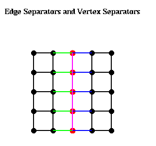
Given an edge separator Es, one can produce a vertex separator Ns by taking one end-point of each edge in Es; Ns clearly has at most as many members as Es. Given a vertex separator Ns, on can produce an edge separator Es by taking all edges incident to Ns; Es clearly has at most d times as many members as Es, where d is the maximum degree (number of incident edges) of any node. Thus, if d is small, finding good edge separators and good vertex separators are closely related problems, a fact we exploit below.
|S| = m = sqrt(m2) = sqrt(number of nodes).It turns out that it is generally possible to find a vertex separtor containing about the square root of the number of nodes.
Theorem. (Tarjan, Lipton, "A separator theorem for planar graphs", SIAM J. Appl. Math., 36:177-189, April 1979). Let G=(N,E) be an planar graph. Then we can find a vertex separator Ns, so that N = N1 U Ns U N2 is a disjoint partition of N, |N1| <= (2/3)*|N|, |N2| <= (2/3)*|N|, and |Ns| <= sqrt(8*|N|).
In other words, there is a vertex separator Ns that separate the nodes N into two parts, N1 and N2, neither of which can be more than twice as large as the other, and Ns has no more than about the square root of the number of nodes. This intuition motivates the algorithms below.
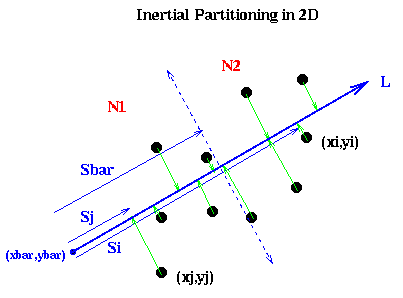
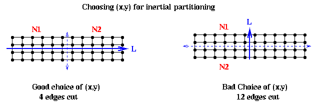
It remains to show how to pick the line L. Intuitively, if the nodes are located in a long, thin region of the plane, as in the above example, we want to pick L along the long axis this region:
In mathematical terms, we want to pick a line such that the sum of squares of lengths of the green lines in the figure are minimized; this is also called doing a total least squares fit of a line to the nodes. In physical terms, if we think of the nodes as unit masses, we choose (x,y) to be the axis about which the moment of inertia of the nodes is minimized. This is why the method is called inertial partitioning. This means choosing a, b, xbar and ybar so that a2 + b2 = 1, and the following quantity is minimized:
     sumi=1,...,|N| (length of i-th green line)2
   = sumi=1,...,|N| ((xi-xbar)2 + (yi-ybar)2 -
                               (-b*(xi-xbar) + a*(yi-ybar))2 )
        ... by the Pythagorean theorem
   =   a2 *   ( sumi=1,...,|N| (xi-xbar)2 )
     + b2 *   ( sumi=1,...,|N| (yi-ybar)2 )
     + 2*a*b * ( sumi=1,...,|N| (xi-xbar)*(yi-ybar) )
   = a2 * X2 + b2 * Y2 + 2*a*b * XY
   = [ a b ] * [ X2  XY ] * [ a ]
               [ XY  Y2 ]   [ b ]
   = [ a b ] * M * [ a ]
                   [ b ]
where X2, Y2 and XY are the summations in the previous lines.
On can show that an answer is to choose
   xbar = sumi=1,...,|N| xi / |N|
   ybar = sumi=1,...,|N| yi / |N|
i.e. (xbar,ybar) is the "center of mass" of the nodes, and (a,b) is the unit eigevector corresponding to the smallest eigenvalue of the matrix M.
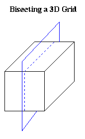
The 3D (and higher) case is similar, except that we get a 3-by-3 matrix whose eigenvector we need.
To extend our intuition about planar graphs to higher dimensions, we need a notion of graphs that are well-shaped in some sense. For example, we might ask that the cells created by edges joining nodes (triangles in 2D, simplices in 3D, etc.) cannot have angles that are too large or too small. The following approach is taken by G. Miller, S.-H. Teng, W. Thurston and S. Vavasis ("Automatic mesh partitioning", in Graph Theory and Sparse Matrix Computation, Springer-Verlag 1993, editted by J. George, J. Gilbert and J. Liu). Our presentation is drawn from "Geometric Mesh Partitioning" by J. Gilbert, G. Miller and S.-H. Teng.
Definition. A k-ply neighborhood system in d dimensions is a set {D1,...,Dn} of closed disks in d-dimensional real space Rd, such that no point in Rd is strictly interior to more than k disks.
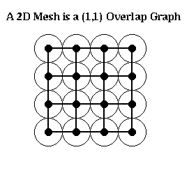
Definition. An (alpha,k) overlap graph is a graph defined in terms of a constant alpha >= 1, and a k-ply neighborhood system {D1,...,Dn}. There is a node for each disk Di. There is an edge (i,j) if expanding the radius of the smaller of Di and Dj by a factor alpha causes the two disks to overlap.
For example, an n-by-n mesh is a (1,1) overlap graph, as shown below. The same is true for any d-dimensional grid. One can show any planar graph is an (alpha,k) overlap graph for suitable values of alpha and k.
One can prove the following generalization of the Lipton-Tarjan theorem:
Theorem. (Miller, Teng, Thurston, Vavasis). Let G=(N,E) be an (alpha,k) overlap graph in d dimensions with n nodes. Then there is a vertex separator Ns, so that N = N1 U Ns U N2, with the following properties:
The separator is constructed by choosing a sphere in d-dimensional space, using the edges it cuts as an edge separator, and extracting the corresponding vertex separator. There is a randomized algorithm for choosing the sphere from a particular probability distribution such that it satisfies the conditions of the theorem with high probability.
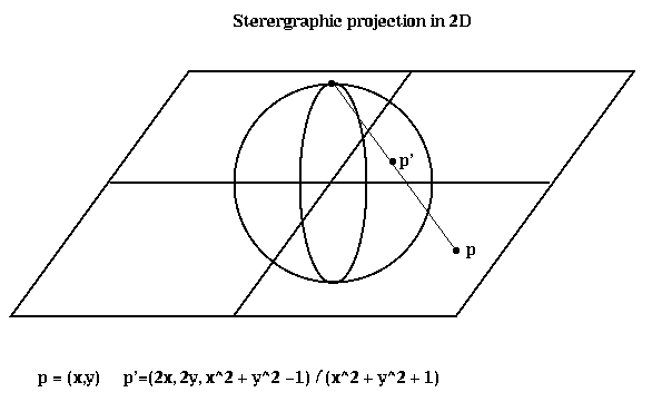
To describe the algorithm, we need to explain stereographic projection, which is a way of mapping points in a d-dimensional space to the unit sphere centered at the origin in (d+1) dimensional space. When d=2, this is done by drawing a line from the point p to the north pole of the sphere; the point p' where the line and sphere intersect is the stereographic projection of p. The same idea applies to higher dimensions.
Here is the algorithm. Matlab software implementing it is available via anonymous ftp from ftp.parc.xerox.com at /pub/gilbert/meshpart.uu.
More recently, a slightly different approach was taken in "Partitioning Meshes with Lines and Planes", by F. Cao, J. Gilbert, and S-H. Teng. Their algorithm is even simpler than the one above, but requires the following slightly different notion of well-shaped graph to analyze. Assume that the node of the graph G have coordinates in Rd, as before.
Let n be a node in G, and let alpha(n) be the ratio
             Euclidean distance from n to the farthest
                   node to which it is connected
  alpha(n) = -----------------------------------------------
             Euclidean distance from n to the nearest other
                   node, whether it is connected to n or not
Note that alpha(n) >= 1.
Then let alpha(G) be the largest value of alpha(n) for any n.
We say that G is an alpha(G)-well-shaped mesh.
One can easily show that there is a bound C(alpha(G),d)
on the largest degree of any node of G, depending only on alpha(G) and d.
If alpha(G) is not much larger than 1, then G looks like a mesh
(in the case of the 2D mesh shown above, it is exactly 1).
Next, we define the trestle D(G) of G as follows. Let m be the shortest length of any edge of G, and M the longest length. Then
D(G) = 1 + log2 (M/m)The idea is that D(G) is the number of significant bits needed to resolve the shortest and longest edges. If all edges are equally long, M=m and D(G) = 1. If the mesh is graded, with long edges in some places and short ones elswhere, D(G) may be large. Such graded meshes are common in finite element applications.
The partitioning algorithm is simply
Finally, Cao, Gilbert and Teng prove the following
Theorem. Let G be an alpha(G)-well-shaped mesh in d dimensions, with n nodes, and with trestle D(G). Then the above algorithm finds a vertex separator Ns, so N = N1 U N2 U Ns, with the following properties:
The implementation requires a data structure called a Queue, or a First-In-First-Out (FIFO) list. It will contain a list of objects to be processed. There are two operations one can perform on a Queue. Enqueue(x) adds an object x to the left end of the Queue. y=Dequeue() removes the rightmost entry of the Queue and returns it in y. In other words, if x1, x2, ..., xk are Enqueued on the Queue in that order, then k consecutive Dequeue operations (possibly interleaved with the Enqueue operations) will return x1, x2, ... , xk.
  NT = {(r,0)}
         ... Initially T is just the root r,
         ...   which is at level 0
  ET = empty set
         ... T = (NT, ET) at each stage of the algorithm
  Enqueue((r,0))
         ... Queue is a list of nodes to be processed
  Mark r
         ... Mark the root r as having been processed
  While the Queue is nonempty
         ... While nodes remain to be processed
      (n,level) = Dequeue()
             ... Get a node to process
      For all unmarked children c of n
         NT = NT U (c,level+1)
                 ... Add child c to the list of nodes NT of T
         ET = ET U (n,c)
                 ... Add the edge (n,c) to the edge list ET of T
         Enqueue((c,level+1))
                 ... Add child c to Queue for later processing
         Mark c
                 ... Mark c as having been visited
      End for
  End while
For example, the following figure shows a graph, as well as the
embedded BFS tree (edges shown
in black). In addition to the tree edges, there are two other kinds of edges.
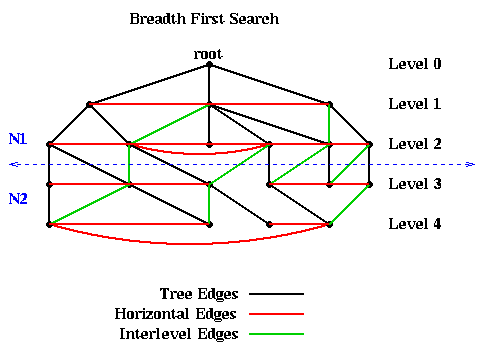
The most important fact about the BFS tree is that there are no edges connecting nodes in levels differing by more than 1. In other words, all edges are between nodes in the same level or adjacent levels. The reason is this: Suppose an edge connects n1 and n2 and that (without loss of generality) n1 is visited first by the algorithm. Then the level of n2 is at least as large as the level of n1. The level of n2 can be at most one higher than the level of n1, because it will be visited as a child of n2.
This fact means that simply partitioning the graph into nodes at level L or lower, and nodes at level L+1 or higher, guarantees that only tree and interlevel edges will be cut. There can be no "extra" edges connecting, say, the root to the leaves of the tree. This is illustrated in the above figure, where the 10 nodes above the dotted blue line are assigned to partition N1, and the 10 nodes below the line as assigned to N2.
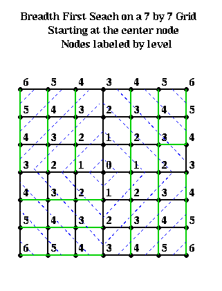
For example, suppose one had an n-by-n mesh with unit distance between nodes. Choose any node r as root from which to build a BFS tree. Then the nodes at level L and above approximately form a diamond centered at r with a diagonal of length 2*L. This is shown below, where nodes are visited counterclockwise starting with the north.
We start with an edge weighted graph G=(N,E,WE), and a partitioning G = A U B into equal parts: |A| = |B|. Let w(e) = w(i,j) be the weight of edge e=(i,j), where the weight is 0 if no edge e=(i,j) exists. The goal is to find equal-sized subsets X in A and Y in B, such that exchanging X and Y reduces the total cost of edges from A to B. More precisely, we let
T = sum[ a in A and b in B ] w(a,b) = cost of edges from A to Band seek X and Y such that
new_A = A - X U Y and new_B = B - Y U Xhas a lower cost new_T. To compute new_T efficiently, we introduce
  E(a) = external cost of a = sum[ b in B ] w(a,b)
  I(a) = internal cost of a = sum[ a' in A, a' != a ] w(a,a')
  D(a) = cost of a = E(a) - I(a)
and analogously
  E(b) = external cost of b = sum[ a in A ] w(a,b)
  I(b) = internal cost of b = sum[ b' in B, b' != b ] w(b,b')
  D(b) = cost of b = E(b) - I(b)
Then it is easy to show that swapping a in A and b in B changes T to
  new_T = T - ( D(a) + D(b) - 2*w(a,b) )
        = T - gain(a,b)
In other words, gain(a,b) = D(a)+D(b)-2*w(a,b) measures the improvement in the
partitioning by swapping a and b.
D(a') and D(b') also change to
  new_D(a') = D(a') + 2*w(a',a) - 2*w(a',b)
          for all a' in A, a' != a

  new_D(b') = D(b') + 2*w(b',b) - 2*w(b',a)
          for all b' in B, b' != b
Now we can state the Kernighan/Lin algorithm (costs show in comments)
(0)   Compute T = cost of partition N = A U B
                             ... cost = O(|N|2)
      Repeat
(1)       Compute costs D(n) for all n in N
                             ... cost = O(|N|2)
(2)       Unmark all nodes in G
                             ... cost = O(|N|)
(3)       While there are unmarked nodes
                             ... |N|/2 iterations
(3.1)         Find an unmarked pair (a,b) maximizing gain(a,b)
                             ... cost = O(|N|2)
(3.2)         Mark a and b (but do not swap them)
                             ... cost = O(1)
(3.3)         Update D(n) for all unmarked n, as though a and b
                   had been swapped
                             ... cost = O(|N|)
         End while
         ... At this point, we have computed a sequence of pairs
         ...     (a1,b1), ... , (ak,bk) and
         ...     gains gain(1), ..., gain(k)
         ... where k = |N|/2, ordered by the order in which
         ... we marked them
(4)      Pick j maximizing Gain = sumi=1...j gain(i)
         ... Gain is the reduction in cost from swapping
         ...    (a1,b1),...,(aj,bj)
(5)      If Gain > 0 then
(5.2)         Update A = A - {a1,...,aj} U {b1,...,bj}
                            ... cost = O(|N|)
(5.2)         Update B = B - {b1,...,bj} U {a1,...,aj}
                            ... cost = O(|N|)
(5.3)         Update T = T - Gain
                            ... cost = O(1)
         End if
     Until Gain <= 0
In one pass through the Repeat loop, this algorithm computes |N|/2 possible pairs of sets A and B to swap, A = (a1,...,aj) and B=(b1,...,bj), for j=1 to |N|/2. These sets are chosen greedily, so swapping ai and bi makes the most progress of swapping any single pair of nodes. The best of these |N|/2 pairs of sets is chosen, by maximizing Gain. Note that some gains may be negative, if no improvement can be made by swapping just two nodes. Nevertheless, later gains may be large, and so the algorithms can escape this "local minimum".
The cost of each step is shown to the right of the algorithm. Since loop (3) is repeated O(|N|) times, the cost of one pass through the Repeat loop is O(|N|3). The number of passes through the Repeat loop is hard to predict. Empirical testing by Kernighan and Lin on small graphs (|N|<=360), showed convergence after 2 to 4 passes. For a random graph, the probability of getting the optimum in one pass appears to shrink like 2|N|/30. A parallel implementation of this algorithm was design by J. Gilbert and E. Zmijewski in 1987.
More recently, other significant improvements to Kernighan/Lin were proposed in ``A fast and high quality multilevel scheme for partitioning irregular graphs'', by G. Karypis and V. Kumar (click here to get this and related papers).