The two main issues in choosing a data layout for Gaussian elimination are
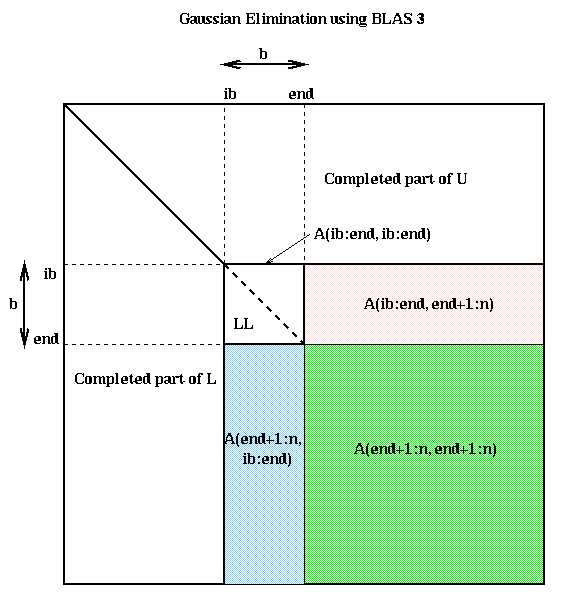
It will help to remember the pictorial representation of Gaussian elimination below. As the algorithm proceeds, it works on successively smaller square southeast corners of the matrix. In addition, there is extra BLAS2 work to factorize the submatrix A(ib:n,ib:end).
For convenience we will number the processors from 0 to p-1, and matrix columns (or rows) from 0 to n-1. The following figure shows a sequence of data layouts we will consider. In all cases, each submatrix is labeled with the number of the processor (from 0 to 3) that contains it. Processor 0 owns the shaded submatrices.
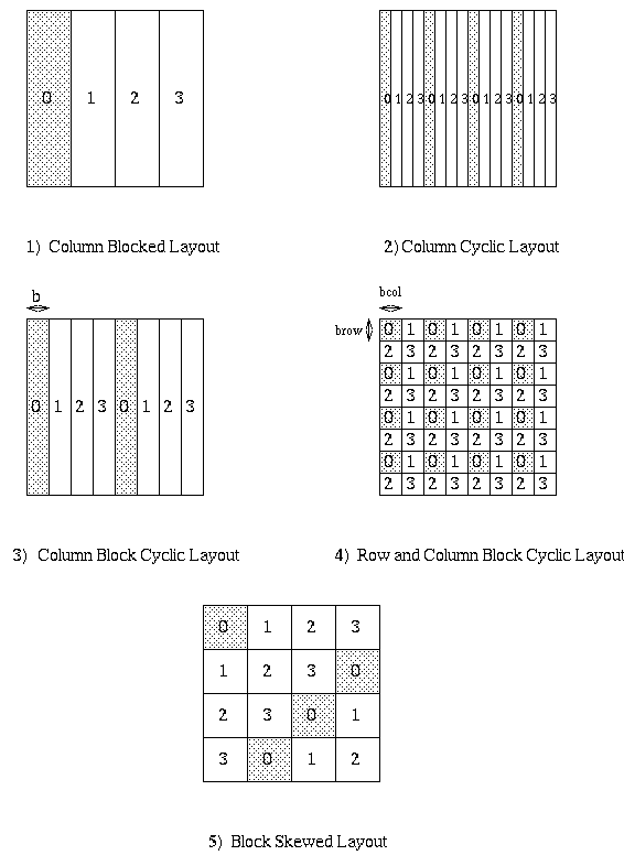
Consider the first layout, the Column Blocked Layout. In this layout, column i is stored on processor floor(i/c) where c=ceiling(n/p) is the maximum number of columns stored per processor. In the figure n=16 and p=4. This layout does not permit good load balancing, because as soon as the first c columns are complete, processor 0 is idle for the rest of the computation. The transpose of the this layout, the Row Blocked Layout, has a similar problem.
The second layout, the Column Cyclic Layout, tried to address this problem by assigning column i to processor i mod p. In the figure, n=16 and p=4. With this layout, each processor owns approximately 1/p-th of the square southeast corner of the matrix, so the load balance is good. However, the fact that single columns are stored rather than blocks means we cannot use the BLAS2 to factorize A(ib:n,ib:end), and may not be able to use the BLAS3 to update A(end+1:n,end+1:n). The transpose of this layout, the Row Cyclic Layout, has a similar problem.
The third layout, the Column Block Cyclic Layout, is a compromise between the last two. We choose a block size b, divide the columns into groups of size b, and distribute these groups in a cyclic manner. This means column i is stored in processor (floor(i/b)) mod p. In fact, this layout includes the first two as the special cases b=c=ceiling(n/p) and b=1, respectively. In the figure n=16, p=4 and b=2. For b larger than 1, this has a slightly worse balance than the Column Cyclic Layout, but can use the BLAS2 and BLAS3. For b less than c, it has a better load balance than the Columns Blocked Layout, but can only call the BLAS on smaller subproblems, and so perhaps take less advantage of the local memory hierarchy (recall our plot of performance of the BLAS3, where performance improved for larger matrix sizes). However, this layout has the disadvantage that the factorization of A(ib:n,ib:end) will take place on perhaps just on processor (in the natural situation where column blocks in the layout correspond to column blocks in Gaussian elimination). This would be a serial bottleneck.
This serial bottleneck is eased by the fourth layout in the figure, the Row and Column (or 2D) Block Cyclic Layout. Here we think of our p processors arranged in an prow-by-pcol rectangular array of processors, indexed in a 2D fashion by (pi,pj), 0 <= pi < prow and 0 <= pj < pcol. All the processors (i,j) with a fixed j are referred to as processor column j. All the processors (i,j) with a fixed i are referred to as processor row i. Matrix entry (i,j) is mapped to processor (pi,pj) by mapping i to pi and j to pj independently using the formula for a block cyclic layout:
    pi = floor(i/brow) mod prow, where
  brow = block size in the row direction

    pj = floor(j/bcol) mod pcol, where
  bcol = block size in the column direction
Thus, this layout includes all the previous layouts, and their transposes,
as special cases. In the figure, n=16, p=4, prow=pcol=2, and brow=bcol=2.
This layout permits pcol-fold parallelism in any column, and calls to the
BLAS2 and BLAS3 on matrices of size brow-by-bcol. This is the layout that
we will use for Gaussian elimination.
Since Gaussian elimination is not
entirely "symmetric" (there is more communication required during
the BLAS2 factorization of A(ib:n,ib:end) than during the BLAS3 update
of A(ib:end,end+1:n)), it is not clear that choosing an entirely
symmetric layout (prow=pcol) is most efficient. Indeed, later we will
see that choosing prow
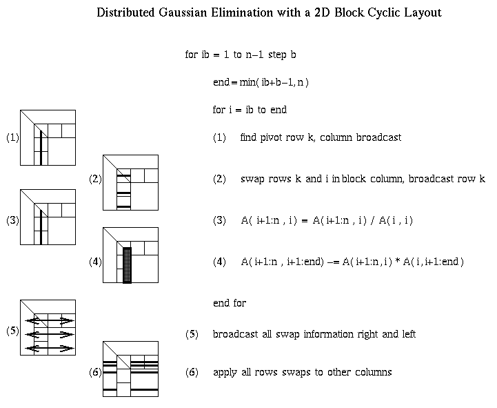
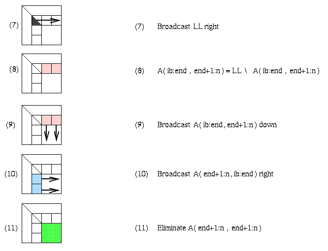
For example, step (1) requires a reduction operation among the prow processors owning the current column, in order to find the largest absolute entry (pivot) and broadcast its index. Step (2) requires communication among processors in that column to exchange rows, and broadcast the pivot row to all processors in the column. Steps (3) and (4) are local computation, BLAS1 and BLAS2, respectively. Steps (5) and (6) involve communication, broadcasting pivot information and swapping rows among all the other p-prow processors. Step (7) is more communication, sending LL to all pcol processors in its row. Step (8) is local computation. Steps (9) and (10) are communication, sending matrix blocks right and down respectively, in preparation for the local matrix multiplies that update the trailing southeast square matrix in step (11).
It is unnecessary to have a barrier between each step of the algorithm. In other words, there can be parallelism with some steps of the algorithm forming a pipeline. For example, consider steps 9, 10 and 11, where most of the communication and floating point work occurs. As soon as a processor received its desired (blue) subblock of A(end+1:n,ib:end) from the left, and (pink) subblock of A(ib:end:end+1:n) from above, it may begin its local matrix multiply to update its part of the (green) submatrix A(end+1:n,end+1:n). As soon as the leftmost b columns of A(end+1:n,end+1:n) are updated, their LU factorization may begin while the remaining columns of the green submatrix are being updated by other processors.
The ScaLAPACK software which implements this is located here. To view the top level routine that performs Gaussian elimination, pdgetrf.f, click here.
   Time =   msgs * alpha
          + words * beta + flops   time units
where msgs is the number of messages sent
(not counting those sent in parallel), words is the number of words sent
(again not counting those sent in parallel), and flops is the number of
floating point operations performed (again, not counting those in parallel).
To make the presentation simple, we will only look at steps 9, 10 and 11 in
detail. It turns out these account for almost all of words and flops,
which are the most important terms for large n.
The implementation we discuss will overlap steps 10 and 11 of the algorithm as described above. More precisely,
To estimate the total cost for Distributed Gaussian Elimination, we need to sum the above three contributions for end = b, 2*b, 3*b, ... , n-b to get Time for all steps 9, 10 11 =
( ( n * (log_2 prow) + 2 ) / b )
* alpha
+ ( n^2 *
( (log_2 prow)/(2*pcol) + 1/prow )
) * beta
+ ( (2/3)*n^3/p )
Taking the other steps of algorithm into account increases the coefficients
of alpha and beta, yielding
 Time for distributed Gaussian elimination =
       ( n * (6+ log_2 prow) ) * alpha
     + ( n^2 *
         ( 2*(prow-1)/p +
           (pcol-1)/p +
           (log_2 prow)/(2*pcol)
         )
       ) * beta
     + ( (2/3)*n^3/p )
We compute the efficiency by dividing the serial time, (2/3)*n^3,
by p times the Time just displayed, yielding
  Efficiency = 1 / (  1
     + (1.5*p*(6 + log_2 prow)/n^2)
       * alpha
     + ( 1.5*
       ( 2*prow + pcol
         + (prow * log_2 prow)/2 -3 )
       /n )
       * beta )(ib:end, end+1:n)
Let us examine this formula, and ask when it is likely to be close to 1,
i.e. when we can expect good efficiency. First, for fixed p, prow, pcol,
alpha and beta, the efficiency approaches 1 as n grows. This is because
we are doing O(n^3) floating point operations, but communicating only O(n^2)
words, so eventually the floating point, which is load balanced, swamps the
communication, so efficiency is good.
The efficiency also grows if alpha and beta shrink, i.e. as communication
becomes less expensive.
Now we consider the choice of prow and pcol. The expression
   2*prow + pcol + (prow * log_2 prow)/2
      = 2*prow +1/prow + (prow * log_2 prow)
is minimized when prow is slightly smaller than sqrt(p), meaning
we want a prow-by-pcol processor grid which is slightly longer than it
is tall. (In practice, for a given p, we are limited to choosing
prow and pcol among the factors of p, unless we want to have idle
processors.)
Overall, assuming prow ~ pcol ~ sqrt(p), and ignoring the log terms, the efficiency is
  Efficiency = 1 / ( 1 + O( p/n^2 * alpha ) +
                  O( sqrt(p)/n * beta ) )
             = E( n^2/p )
i.e. an increasing function of n^2/p. But n^2/p is the amount of
data stored per processor, since an n-by-n matrix takes up n^2 words.
In other words, if we let the "total problem size" n^2 grow proportionally
to the number of processor, we expect the efficiency to be approximately
constant. Let us confirm this hypothesis with an experiment.
We will use the Intel Gamma, which has the following machine parameters:
Click here for the predicted run times on the Gamma, and click here for the actual run times; they are satisfyingly close together, and confirm that the efficiency is to first order simply an increasing function of n^2/p. The predicted times are labelled by the memory used per processor in Megabytes, ranging from 2 to 6.25.