CS267: Lecture 1, Jan 16 1996
Introduction to Parallel Computing
Introduction
We will have much class material available on the World Wide Web (WWW),
accessed via
Netscape or
Mosaic:
The
first handout
describes the course organization in more detail. Here is an overview of the course.
Parallel Machines
We will discuss a variety parallel and other high performance computer
architectures, though not in as much detail as the
Parallel Architecture class CS258, or as the
on-line documentation available on the
class home page.
We will discuss a few historically
important architectures, and describe trends in the industry.
Architectures have been changing rapidly over the last few years,
and while there is some convergence, it is quite likely you will continue to
have to know a reasonable amount about an architecture to use it effectively.
The parallel and/or high performance machines available to us this semester include:
Programming Languages
There is no standard parallel programming language, any more than there is
a standard serial programming language. There are computer architecture specific
languages, application specific languages, general purpose languages, and a
variety of tools and libraries available. Some languages try to make many
optimization decisions for the user (and so may make poor decisions),
and others leave most of the details to the user (so more programming effort
is required, but performance may be much better).
Few reliable or commercial products are available;
we will try to give an overview of this rapidly changing area.
The languages we will use include:
Libraries for Parallel Machines
A number of parallel subroutine libraries have been written, in an attempt to
provide good implementations of certain common problems. Some of these libraries
are portable across different parallel architectures, and others are not.
The list below mentions those we expect to discuss this semester
(it will be updated throughout the semester).
We will try to emphasize programming tools that have a future
(including but not limited to our own), or at least interesting ideas.
Applications and related algorithms
We will use a collection of programs called
Sharks and Fish,
which simulate fish and sharks swimming around,
eating, breeding, and dying, while obeying rules which model more
complicated and realistic force fields.
Sharks and Fish provide a simple model of
particle simulations, such as
ions in a plasma, cars on a freeway, stars in a galaxy, etc.
We have implemented a variety of sharks-and-fish simulations in the major
programming languages listed above, so we can easily compare how different
languages express parallelism. Your assignments will include making
modifications to these programs.
We will discuss algorithms for linear algebra problems, such as
solving linear systems of equations and finding eigenvalues. These
arise in applications from many fields (including structural mechanics,
circuit simulation, computational chemistry, etc.). We will cover
methods for both dense and sparse matrices, and direct and
iterative methods (for example, Gaussian elimination and conjugate gradients,
respectively). Many of these algorithms have been implemented in the
libraries discussed above.
These linear algebra problems often arise from solving
differential equations, which arise in many areas. We will
discuss the heat equation, Poisson's equation, and
equations involved in climate modeling in particular.
We will also discuss variety of more complicated applications,
which require complicated distributed data structures,
or combining various of the earlier techniques we discussed.
The list of applications includes circuit simulation,
solving systems of polynomial equations algebraically,
cell simulation, computational genetics, game search,
and electromagnetic field simulation. The choice will depend
on the interest of the class.
Combinatorial problems such as sorting, computing connected components
of a graph, and the Traveling Salesman Problem will also be discussed.
Motivation for Parallel Computing
The
traditional scientific paradigm is first to do theory (say on paper),
and then lab experiments to confirm or deny the theory. The
traditional engineering paradigm is first to do a design (say on paper),
and then build a laboratory prototype.
Both paradigms are being replacing by numerical experiments and
numerical prototyping. There are several reasons for this.
Scientific and engineering problems requiring the most computing power to
simulate are commonly called "Grand Challenges"
Click on
Grand Challenges or
largest problems,
like predicting the climate 50 years hence, are
estimated to require computers computing at the rate of 1 Tflop =
1 Teraflop = 10^12 floating point operations per second, and with a
memory size of 1 TB = 1 Terabyte = 10^12 bytes.
Here is some commonly
used notation we will use to describe problem sizes:
       1 Mflop = 1 Megaflop = 10^6 floating point operations per second
       1 Gflop = 1 Gigaflop = 10^9 floating point operations per second
       1 Tflop = 1 Teraflop = 10^12 floating point operations per second
       1 MB    = 1 Megabyte = 10^6 bytes
       1 GB    = 1 Gigabyte = 10^9 bytes
       1 TB    = 1 Terabyte = 10^12 bytes
       1 PB    = 1 Petabyte = 10^15 bytes
Let us illustrate how these problems could require such large computing
resources. We will consider climate modeling in particular, using a vastly
oversimplied model of a system being developed under NASA support at
UCLA and
Berkeley.
What is climate? Mostly simply, it is a function of 4 arguments
Climate (longitude,latitude,elevation,time)
which returns a vector of 6 values:
temperature, pressure, humidity, and wind velocity(3 words).
(More generally, we could ask for the concentration of each chemical
species, such as ozone, in addition to the 6 values above.)
To represent this continuous function
in the computer we need to discretize, or only evaluate
climate for the arguments lying on a grid: Climate(i,j,k,n), where t = n*dt,
dt a fixed time step, n an integer, and i,j,k are integers indexing the
longitude, latitude and elevation grid cells, respectively.
(A real model has to have equations for all the other atmospheric
processes too, such as cloud formation, precipitation, chemistry, etc.).
An algorithm to predict the weather (short term) or climate (long term, and
only statistically significant),
is a function which maps the climate at time t,
Climate(i,j,k,n), for all i,j,k, to the climate at the next time step t+dt,
Climate(i,j,k,n+1), for all i,j,k.
The algorithm involves solving a system of
equations including, in particular the Navier-Stokes equations for fluid flow
of the gasses in the atmosphere.
Suppose we discretize the earth's surface into 1 kilometer-by-1 kilometer cells in the
latitude-longitude direction, and with 10 cells in the vertical direction. From
the surface area of the earth, we can compute that there are about
5e9 ( = 5 x 10^9) cells in the atmosphere. With six 4-byte words per cell,
that comes to about 10^11 = .1 TB (to the nearest order of magnitude).
Suppose we take 100 flops (floating point operations) to update each cell
by one minute. In other words, dt = 1 minute, and computing Climate(i,j,k,n+1)
for all i,j,k from Climate(i,j,k,n) takes about 100*5e9 = 5e11 floating point
operations. It clearly makes no sense to take longer than one minute to
predict the weather one minute from now; otherwise it is cheaper to look out
the window. Thus, we must compute at least at the rate of
5e11 flops / 60 secs ~ 8 Gflops.
Weather prediction (computing 24 hours to compute the weather 7 days hence)
requires computing 7 times faster, or 56 Gflops. Climate prediction (computing
30 days, a long run, to compute the climate 50 years hence), requires computing
50*12=600 times faster, or 4.8 Tflops.
The actual grid resolution used in climate codes today is 4 degrees
of latitude by 5 degrees of longitude, or about 450 km by 560 km,
a rather coarse resolution. A near term goal is to improve this resolution
to 2 degrees by 2.5 degrees, which is four times as much data.
The size of the overall database is enormous. NASA is putting up weather satellites
expected to collect 1TB/day for a period of years, totaling as much as 6 PB of
data, which no existing system is large enough to store. The
Sequoia 2000 Global Change Research Project is concerned with building
this database.
Why parallelism is essential
The speed of light is an intrinsic limitation
to the speed of computers. Suppose we wanted to build a completely sequential
computer with 1 TB of memory running at 1 Tflop. If the data has to travel
a distance r to get from the memory to the CPU, and it has to travel this
distance 10^12 times per second at the speed of light c=3e8 m/s,
then r <= c/10^12 = .3 mm. So the computer has to fit into a box .3 mm on a
side.
Now consider the 1TB memory. Memory is conventionally built as a planar grid
of bits, in our case say a 10^6 by 10^6 grid of words. If this grid
is .3mm by .3mm, then one word occupies about 3 Angstroms by 3 Angstroms,
or the size of a small atom. It is hard to imagine where the wires would go!
Why writing fast programs is hard.
In the Netlib repository
there is a long list of ``all'' computers, together with
performance benchmark information.
One benchmark, the
Linpack Benchmark,
sorts all machines by the speed with which they can solve systems of linear
equations Ax=b, of various dimensions, using Gaussian elimination.
As of Jan 1996, the fastest machine is an Intel Paragon with
6768 processors and a peak speed of 50 Mflops/proc, for an overall
peak speed of 6768*50 = 338 Gflops. Doing Gaussian elimination, the machine
gets 281 Gflops on a 128600x128600 matrix; the whole problem takes 84min.
This is also a record for the largest dense matrix solved by Gaussian
elimination (a record which has held for a year, a long time in this business).
Current Paragons have i860 chips, but future Paragons may have
Pentiums (hopefully ones that do division correctly).
But, if we try to solve a much tinier 100-by-100 linear system, the fastest the
system will go is 10 Mflops rather than 281 Gflops, and that is attained using
just one of the 6768 processors, an expensive waste of silicon. Staying with
a single processor, but going up to a 1000x1000 matrix, the speed goes up to
36 Mflops.
Where do the flops go? Why does the speed depend so much on the problem size?
The answer lies in understanding the memory hierarchy.
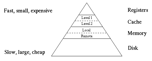
All computers, even cheap ones, look something like this:
 The memory at the top level of this hierarchy, the registers, is small, fast
and expensive. The memory at the bottom level of the hierarchy, disk, is
large, slow and cheap (relatively speaking!). There is a discontinuous change
in size, speed and cost from level to level.
Useful work, such as floating point operations, can only be done on
data at the top of the hierarchy. So to work on data stored lower in the
hierarchy, it must first be transferred to the registers, perhaps displacing
other data already there.
Transferring data among levels is slow, much slower than the rate at which
we can do useful work on data in the registers.
In fact, this data transfer is the bottleneck in most computations:
more time is spent moving data in the hierarchy than doing useful work.
Good algorithm design requires keeping active data near the top
of the hierarchy as long as possible, and minimizing movement
between levels. For many problems, like Gaussian elimination, only if
the problem is large enough is there enough work to do at the top of
the hierarchy to mask the time spent transferring data among lower
levels. The more processors one has, the larger the problem has to be
to mask this transfer time. We will study this example in detail later.
It is often remarked that speeds of basic microprocessors grow by a factor of 2
every 18 months; this empirical observation, true over many years, is called
Moore's Law. In case you think that parallel programming is too hard,
and that you would rather wait until Moore's Law makes the personal computer
on your desk fast enough for your problem, think again: The reason Moore's Law
is true, is that microprocessor manufacturers are adopting many of the tricks of
parallel computing and accounting for memory hierarchies that we will discuss.
So getting the peak speed from your microprocessor is becoming more difficult.
There is no way around the issues we will discuss.

