The IEEE floating point standards prescribe precisely how floating point numbers should be represented, and the results of all operations on floating point numbers. There are two standards: IEEE 754 is for binary arithmetic, and IEEE 854 covers decimal arithmetic as well. We will only discuss IEEE 754, which has been adopted almost universally by computer manufacturers. Indeed, except for older, obsolete architectures (such as IBM 370 and VAX), and the Cray XMP, YMP, 2, C90 and first generation T90, all other machines, including PCs, workstations, and parallel machines built from the same microprocessors, use IEEE arithmetic. The next Cray T90 will also implement IEEE arithmetic.
So the good news is that essentially all new computers will be using the same floating point arithmetic in the near future, and almost all do now, with the important exception of Cray. This simplifies code development, especially portable code development, as well as some important rounding error analyses, as we will illustrate below.
Unfortunately, not all manufacturers implement every detail of IEEE arithmetic the same way. Everyone does indeed represent numbers with the same bit patterns, and rounds results correctly (or tries to!). But exceptional conditions (like 1/0, sqrt(-1) etc.), whose semantics are also specified in detail by the IEEE standard, are not always handled the same way. It turns out that many manufacturers believe (sometimes rightly and sometimes wrongly) that conforming to every detail of IEEE arithmetic would make their machines either a bit slower or a bit more expensive, enough so make them less attractive in the marketplace. In particular, machines are often sold on the basis of how fast they execute certain standard benchmarks, like the Linpack Benchmark, which do not generate exceptions, so exception handling often gets short shrift. We will discuss the impact of this on code development.
                              Floating point formats

Name of format   Bytes to  Number of bits       Macheps      Number of        Approx range
                 store     in significand                    exponent bits
--------------   --------  --------------       -------      -------------    ------------
Single              4            24          2^(-24) ~ 1e-7        8            10^(+-38)
Double              8            53          2^(-53) ~ 1e-16      11          >=10^(+-308)
Double extended  >=10          >=64        <=2^(-64) ~ 1e-19    >=15          >=10^(+-4932)
Quadruple          16           113          2^(-113)~ 1e-34      15            10^(+-4932)
Macheps is short for "machine epsilon", and is used below for roundoff error analysis.
The distance between 1 and the next larger floating point number is 2*macheps.
When the exponent has neither its largest possible value (a string of all ones) nor its smallest possible value (a string of all zeros), then the significand is necessarily normalized, and lies in [1,2).
When the exponent has its largest possible value (all ones), the floating point number is either +infinity, -infinity, or NAN (not-a-number); we discuss these further below under exceptions. The largest finite floating point number is called the overflow threshold.
When the exponent has its smallest possible value (all zeros), the significand may have leading zeros, and is called either subnormal or denormal (unless it is exactly zero). The subnormal floating point numbers represent very tiny numbers between the smallest nonzero normalized floating point number (the underflow threshold) and zero. An operation that underflows yields a subnormal number or possibly zero; this is called gradual underflow. The alternative, simply returning a zero, is called flush to zero. When the significand is zero, the floating point number is +-0.
The basic operations specified by IEEE arithmetic are first and foremost addition, subtraction, multiplication and division. Square roots and remainders are also included. The default rounding for these operations is "to nearest even". This means that the floating point result fl(a op b) of the exact operation (a op b) is the nearest floating point number to (a op b), breaking ties by rounding to the floating point number whose bottom bit is zero (the "even" one). It is also possible to round up, round down, or truncate (round towards zero). Rounding up and down are useful for interval arithmetic, which can provide guaranteed error bounds; unfortunately most languages and/or compilers provide no access to the status flag which can select the rounding direction.
Other operations include binary-decimal conversion, floating point-integer conversions, and conversions among floating point formats, and comparisons.
(*) fl(a op b) = (1+ eps)*(a op b) provided fl(a op b) neither overflows nor underflowswhere
      (a op b) is the exact result of the operation, where op is one of +, -, * and /
      fl(a op b) is the floating point result
      | eps | <= macheps
To incorporate underflow, we may write
fl(a op b) = (1+ eps)*(a op b) + eta provided fl(a op b) does not overflowwhere
| eta | <= macheps * underflow_thresholdOn machines which do not implement gradual underflow (including some IEEE machines which have an option to perform flush-to-zero arithmetic instead), the corresponding error formula is
| eta | <= underflow_thresholdi.e. the error is 1/macheps times larger.
(**)  fl(a +- b) = ( (1+eps1)*a ) +- ( (1+eps2)*b )    provided fl(a +- b ) neither overflows
                                                       nor underflows
In particular, this means that if a and b are nearly equal, so a-b is much smaller than
either a or b (this is called extreme cancellation),
then the relative error may be quite large. For example when subtracting
1-x, where x is the next smaller floating point number than 1, the answer is twice too
large on a Cray C90, and 0 when it should be nonzero on a Cray 2.
This happens because when y's significand is shifted right to line its binary point up with 1's binary point, prior to actually subtracting the significands, any bits shifted past the least significant bit of 1 are simply thrown away (differently on a C90 and Cray 2), rather than participating in the subtraction. On IEEE machines, there is a so-called guard digit (actually 3 of them) to store any bits shifted this way, so they can participate in the subtraction.
This source of error has little effect on most problems in numerical linear algebra, but there are some important exceptions, as illustrated below.
error = alg(x) - f(x)Rather than trying to compute the error directly, we proceed as follows.
We first try to show that alg(x) is numerically stable, that is alg(x) is nearly the exact result f(x+e) of a slightly perturbed problem x+e:
alg(x) ~ f(x+e) where e is small
Second, assuming f(x) is a smooth function at x, we approximate f(x) by a first-order Taylor expansion near x:
f(x+e) ~ f(x) + e*f'(x)
Combining the last two expressions yields
         error = alg(x) - f(x)
               ~ f(x+e) - f(x)
               ~ f(x) + e*f'(x) - f(x)
               = e*f'(x)
Thus, we have expressed the error as a product of a small quantity e and the derivative
f'(x). e is usually called the backward error of the algorithm. f'(x), which
depends only on f and not on the algorithm, is called the condition number.
In other words, the error is approximately the product of the backward error and
the condition number. This approach is ubiquitous in numerical linear algebra,
where x and f(x) are usually vectors and/or matrices, and we use norms to bound the
error:
|| error || <~ || e || * || f'(x) ||Computing || f'(x) || exactly is often as expensive as solving the original problem. Therefore we often settle for an approximation; this is called condition estimation.
Roundoff error analysis is needed to show that e is small. We illustrate with a few examples.
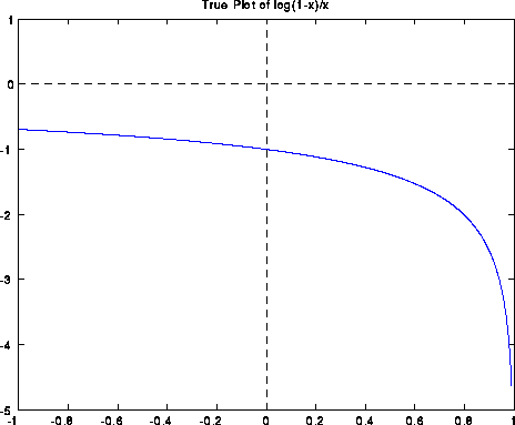
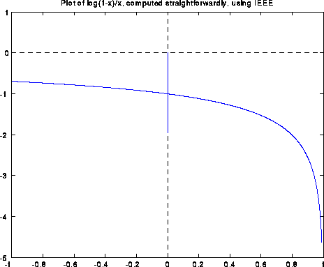
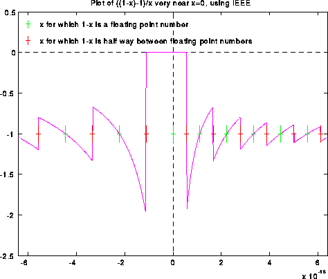
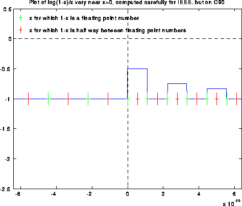
If we evaluate log(1-x)/x in IEEE floating point arithmetic using this formula (except for the special case f(0)=-1), the computed graph is shown below. Note that the answer is quite wrong near x=0, with a spike going from -2 to 0:
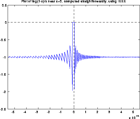
Blowing up the graph near x=0 shows a sort of periodic behavior:
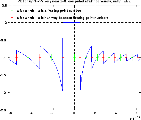
Blowing the graph up even more yields the following picture. To hint at what is going on, we have made green tic marks at all x values such that 1-x is an exact floating point number. The red tic marks are exactly half way in between the green tic marks, and are the thresholds where fl(1-x) suddenly changes from one floating point value to the next.
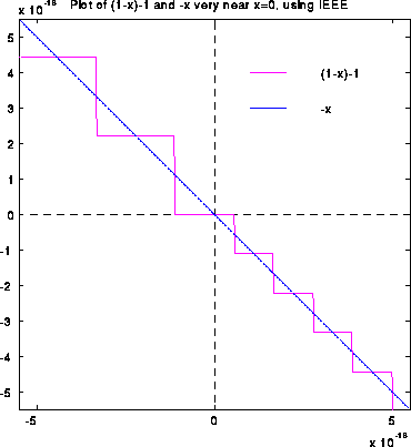
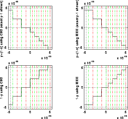
When x is tiny, log(1-x) is very close to -x. Said another way, when y is very close to 1, log(y) is very close to y-1. The next graph shows ((1-x)-1)/x, as computed in floating point. In exact arithmetic, this expression simplies to -1. But in floating point, it yields exactly the same picture as before:
The next graph shows both (1-x)-1 and -x (both computed in floating point) on the same graph. Their quotient is what was shown in the last graph. It is easy to see why the quotient is far from -1: When x is tiny, fl(1-x) can only take on a few discrete values near 1, so fl(fl(1-x)-1) can in turn only take on a few discrete values, whereas x more nearly takes on a continuum of values.
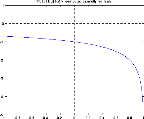
Here is a different algorithm for f(x) which computes it quite precisely in IEEE arithmetic:
       y=1-x
       if y == 1,
          f = -1
       else
          f = log(y)/(1-y)
       endif
In real arithmetic, the algorithm is clearly equivalent to f = log(1-x)/x (except at x=0, where
it has the right limiting value). The graph of this function is shown below; it has no
difficulty near x=0.
This algorithm is backward stable, because it nearly computes log(1-(x+e))/(x+e), where e is small (on the order of of macheps); this makes the very reasonable assumption that the logarithm function is implemented accurately (this is not difficult). We invite the reader to supply a proof. (Hint: when x is small, there is no roundoff error committed when computing fl(1-y).)
Unfortunately, this improved algorithm is not backward stable on the Cray C90, as illustrated in the graph below, which only shows the graph for x near 0:
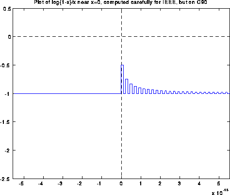
The subsequent plot is a bigger blowup near x=0, with floating point numbers of the form 1-x marked as before.
The following plots show intermediate results in the computation, both on an IEEE machine and on the Cray, for contrast. The final result on an IEEE machine is the quotient of the two values plotted in the two rightmost graphs; their quotient is clearly -1. The final result on a C90 is the quotient of the two values plotted in the two leftmost graphs; their quotient is clearly not -1 for x>0.
The problem lies in the fact that fl(1-y) is off by a factor of up to 2 when y is near 1 on a C90, whereas fl(1-y) is exact in IEEE arithmetic. The cure on a C90 is to replace
y = 1-x
by
y = .5 + (.5 - x)
and
f = log(y)/(1-y)
by
f = log(y)/(.5+(.5-y))
The reader is invited to prove why this works, and to rejoice that the imminent
universality of IEEE arithmetic will make such tricks unnecessary.
Example 2: Finding Eigenvalues by Divide-and-Conquer
Currently the fastest algorithm for finding all eigenvalues and all eigenvectors of
a symmetric matrix on a single processor cache-based machine is based on a divide-and-conquer
approach originally proposed by Cuppen in 1981, and much refined since then. At its heart
is an algorithm for inexpensively computing the eigenvalues and eigenvectors of a matrix
in the special form D + r*z*z', where D is diagonal, r is a scalar, z is a vector, and z' is
the transpose of z. We also call this the diagonal plus rank-one eigenproblem.
The eigenvalues are found by applying a sophisticated version of Newton's method to find the
zeros of a rational function which has the same zeros as the characteristic polynomial.
Given the eigenvalues, the question is how to compute the eigenvectors. There is an
easily confirmed formula for the eigenvector corresponding to a computed eigenvalue lambda,
namely
x = ( D - lambda*I )^(-1) * z
Unfortunately, this formula is quite inaccurate when there are other eigenvalues
very close to lambda. In particular, eigenvectors of different, but nearby, eigenvalues are
not guaranteed to be orthogonal, which is essential for stability.
This difficulty was attacked by Sorensen, Tang, Kahan and others, and proposed solutions were
based on using double the input precision for certain critical parts of the calculation.
When the input precision is already double, this would require quadruple, which is not
widely available; this was the major stumbling block to widespread adoption of this algorithm
for many years.
Finally, in 1992 Eisenstat and Gu nearly completely overcame this problem by using a different,
stable formula, now incorporated in LAPACK routine SSTEDC (and SLAED3, which SSTEDDC calls).
We defer to a later lecture for details of this algorithm, but just examine the kernel
of their formula
x(i) = prod_{j=1 to n except i} q(i,j) / ( lambda(i) - lambda(j) )
where q(i,j) is some other (accurately) computed quantity. Stability depends on this
formula being evaluated accurately.
With IEEE arithmetic we may apply error analysis formula (*) above.
Assuming for simplicity that q(i,j) is exact, we see that the computed x(i)
differs from the true x(i) by a factor f, where f is the product of 2n-1 different terms
of the form 1+eps, |eps| <= macheps. Thus x(i) is computed to high relative accuracy
as desired.
With Cray arithmetic, on the other hand, if some difference lambda(i) - lambda(j)
undergoes extreme cancellation, it may not be computed accurately. If q(i,j) is also
small, the factor q(i,j) / ( lambda(i) - lambda(j) ) may be O(1) and completely
wrong, so that x(i) is completely wrong. This can indeed occur, and this temporarily
prevented us from incorporating divide-and-conquer into LAPACK, until we figured out
what to do.
The fix for this problem was proposed by W. Kahan, who pointed out that if no lambda(i)
has a nonzero least significant bit, then when extreme cancellation occurs no information
is lost by shifting. Thus, simply setting the bottommost bit of each lambda(i) to zero,
a tiny error, would fix the problem. Doing this in a portable way, that would run whether
compiled on a Cray, PC or any other machine, required the following trick: It turns out that
computing
lambda = ( lambda + lambda ) - lambda
has no effect on lambda on any binary machine which rounds in any reasonable way (barring
overflow). But on a Cray, it makes the bottom bit of lambda zero; the reader is invited
to show why.
This still does not explain the ultimate appearance of the LAPACK code. It turns out that
many aggressive optimizing compilers will examine the expression above, and simply throw
it away, because in exact arithmetic, it obviously would have no effect. To try to
prevent this, (lambda+lambda) is actually computed by a function call, where the function
is compiled at a lower level of optimization. This is still no guarantee, but we hope that
by the time compilers become aggressive enough for this to be a problem, non-IEEE arithmetics
will have disappeared.
As a historical note, for a while we considered implementing this algorithm in
doubled precision which represents double precision quantities as
a pair (upper,lower) of single precision quantities, and manipulates these pairs.
The attraction is that if the input precision is already double, this simulates
quadruple, letting us use the same algorithm in all precisions. Algorithms for
this simulation are well known, but require a guard digit
during addition and subtraction to be reasonably efficient. So the Cray's lack of a
guard digit made this approach unattractive too.
Example 3: Computing x/sqrt(x^2+y^2)
A colleague once wrote a Cray program containing the expression
z = arccos( x/sqrt(x^2+y^2) )
An enigmatic run-time error was generated, which he (and several company engineers)
finally tracked down to the fact that the computed value of x/sqrt(x^2+y^2) exceeded 1,
to which arccos() subsequently objected. This occurred on the Cray because of
sloppy rounding in the multiplication, division, and square root functions. Barring
over/underflow, it can not occur using IEEE arithmetic. The user is invited to find a proof.
References for Error Analysis and Numerical Stability
Exception Handling
When the result of a floating point operation is not representable as a
normalized floating point number, and exception occurs. Before the IEEE standard,
machines responded to exceptions in diverse ways, most causing the program to abort,
but some continuing to compute using some default result. Programs that purported to
be both robust and portable therefore had to assume the worst, that exceptions were
invariably fatal, and so use defensive programming techniques that tried to anticipate
most possible sources of exceptions and account for them ahead of time. LAPACK is
constructed this way, for example. The price is slow, complicated, and therefore
harder to maintain software. For example, there is a 700 line subroutine (slatrs.f)
designed to solve triangular systems of linear equations safely no matter how ill-conditioned
or ill-scaled the problem; this routine is used in condition estimation.
A main contribution of IEEE arithmetic was to standardize on how exceptions are handled.
There are five kinds of exceptions, as listed in the table below. The default response
for all 5 types is to set a sticky status flag, and continue computing the the
default result listed below. The status flag can be read by the user, and remains set
until reset by the user (hence "sticky").
Exception Name Cause Default Result
-------------- ----- --------------
Overflow Result too large to represent Return +-Infinity
as a normalized number
Underflow Result too small to represent Return subnormal
as a nonzero normalized number number or 0
Divide-by-zero Computing x/0, where x is Return +-infinity
finite and nonzero
Invalid infinity-infinity, 0*infinity, NAN
infinity/infinity, 0/0, sqrt(-1),
x rem 0, infinity rem y,
comparison with NAN,
impossible binary-decimal conversion
Inexact A rounding error occurred rounded result
Alternatively, the IEEE standard recommends, but does not mandate, an alternative
response to an exception, namely trapping. This means interrupting execution
and jumping to another piece of code, possibly written by the user. In other words,
it does not merely mean jumping to the operating system, printing an error message,
and stopping, although this is indeed what most systems do. In principle, one could
branch to an entirely different algorithm to solve the problem, and continue
computing. The default response and sticky flags also provide this capability, but
the user must check for exceptions and branch explicitly.
This is the area where the most liberties are taken with implementations of IEEE
arithmetic, since a complete implementation of all IEEE recommendations could
impact programming languages, compilers, and operating systems. Also, interrupting
precisely when an operation occurs is very difficult, when many operations are in
partial state of execution in a pipelined execution unit; one either needs to have
a complex enough system to back out of all the partially executed operations, or
abandon many effective forms of pipelining.
Writing faster numerical code using exception handling
Using either sticky flags or traps, it is possible to exploit the following simple paradigm
to write fast, reliable software with IEEE arithmetic. It assumes we have two algorithms
available for a problem, a fast, usually accurate, but occasionally unstable algorithm,
and a slower, more reliable algorithm.
- Use the fast algorithm to compute an answer; this will usually be accurate.
- Quickly and reliably assess the accuracy of the computed answer.
- In the unlikely event that the answer is not good enough, recompute it using
the reliable algorithm.
The utility of this paradigm depends on there being a big difference in speed between
the two algorithms, on being able to assess the accuracy quickly and reliably, and
instabilities in the fast algorithm not causing the program to abort or run very
slowly. This is where IEEE arithmetic comes in: we assume that instabilities,
if they occur, result in a status flag being set (which we can check in step 2),
along with either a trap, or infinities and NaNs propagating harmlessly (and quickly!)
through the computation.
We illustrate this paradigm with two examples below. It is effective on many machines,
except that on machines which implement arithmetic with infinities and NANs very slowly,
the worst case running time (as opposed to the average), could be quite slow.
See the paper by Demmel and Li in the references for details.
Example 4: Condition Estimation
To compute an error bound for the solution of a linear system of equations Ax=b,
we need an estimate of the condition number of A, ||A||*||inv(A)||, where
||.|| is some matrix norm. One may then approximately bound the error in the
computed solution x by
|| computed x - true x ||
------------------------- <= ||A|| * ||inv(A)|| * macheps
|| computed x ||
The problem is to estimate || inv(A) || without computing inv(A) explicitly,
which would usually be more expensive than solving Ax=b in the first place.
LAPACK and other packages use an optimization approach which attempt to find
a unit vector z, such that || inv(A)*z || is as large as possible; this typically
requires a handful of solutions of linear systems of the form A*y=z, for carefully
chosen z vectors. If we have already done Gaussian elimination and factored
the matrix A into the product A=L*U of triangular matrices, the extra work involved in
condition estimation is usually negligible.
Thus, the inner loop of the algorithm requires the solution of triangular linear systems
(with matrices L and U), where we expect the solution to be large. This is where exceptions
come in. When A is nearly singular, so the computed solution is quite large, overflows
are most likely. But if A is nearly singular, this is precisely when the user is most likely
to want to do condition estimation. Therefore, we cannot simply call the existing,
manufacturer-supplied, highly-optimized triangular system solver, because it may overflow.
Therefore, in LAPACK we call our own complicated, slow and reliable alternative slatrs.f,
which is careful to scale inside the inner loop to avoid possible exceptions.
Applying our three-point paradigm to this situation yields the algorithm
- Do condition estimation using a highly-optimized but overflow-susceptible
triangular system solver.
- Check the exception status flags; if no exception occurred, fine.
- Otherwise, recompute using slatrs, or simply signal that the matrix is
highly ill-conditioned.
Thus, in this special case, we can even dispense with the slow reliable code altogether,
since any very large condition number gives as much information to the user as any other
("your computed solution is completely unreliable").
The result is an algorithm which is 1.5 to 5 times faster than the old one on a Sun 4/260,
1.6 to 9.3 times faster on a DEC Alpha, and 2.55 to .421 times faster on a Cray C90.
A Cray C90 does not have IEEE exception handling, but these speedups were obtained in
the most common case where no exceptions occurred. Thus, for the Cray, it measures
the speed penalty paid on Cray by not having exception handling.
Example 4: Finding Eigenvalues Using Bisection
Bisection is a standard serial and (more importantly) parallel algorithm for finding
finding eigenvalues of symmetric tridiagonal matrices. If T is an n-by-n tridiagonal
matrix
[ a(1) b(1) ]
[ b(1) a(2) b(2) ]
T = [ ... ... ... ]
[ b(n-1) a(n-1) b(n) ]
[ b(n) a(n) ]
and s is a shift, then barring exceptions the following simple algorithm counts the
number of eigenvalues of T less than s:
count = 0
b(0) = 0
d = 1
for i = 1 to n
d = a(i) - s - b(i-1)^2/d
if (d<0) count = count + 1
end for
To make this code robust, we must take into account exceptions in the inner loop.
For example, if s were an eigenvalue of the leading k-by-k submatrix of T, then
(in exact arithmetic) the k-th value of d would be exactly zero.
Assuming we prescale T so its largest entry is neither too large nor too small
(making ||T|| equal to the fourth root of the overflow threshold is a good value),
then the following code is robust across all machines, and is currently in LAPACK
routine slaebz.f:
count = 0
b(0) = 0
d = 1
pivmin = sqrt(underflow_threshold)
for i = 1 to n
d = a(i) - s - b(i-1)^2/d
if (abs(d) < pivmin) d = -pivmin ... guarantees division by |d| not too small
if (d < 0) count = count + 1
end for
However, this runs about 14% to 47% slower than the simpler algorithm above. With IEEE
arithmetic, it turns out that the first algorithm is perfectly correct even when d becomes
zero. The result is that the next d will be +-infinity, and on the subsequent iteration
-b(i-1)^2/d will be zero again. One can show that this yields accurate and reliable
results; see the reference below.
References for Exception Handling
In addition to
CS 267 Lecture 21,
see