The implementation requires a data structure called a Queue, or a First-In-First-Out (FIFO) list. It will contain a list of objects to be processed. There are two operations one can perform on a Queue. Enqueue(x) adds an object x to the left end of the Queue. y=Dequeue() removes the rightmost entry of the Queue and returns it in y. In other words, if x1, x2, ..., xk are Enqueued on the Queue in that order, then k consecutive Dequeue operations (possibly interleaved with the Enqueue operations) will return x1, x2, ... , xk.
  NT = {(r,0)}                            ... Initially T is just the root r, which is at level 0
  ET = empty set                          ... T = (NT, ET) at each stage of the algorithm
  Enqueue((r,0))                          ... Queue is a list of nodes to be processed
  Mark r                                  ... Mark the root r as having been processed
  While the Queue is nonempty             ... While nodes remain to be processed
      (n,level) = Dequeue()               ... Get a node to process
      For all unmarked children c of n
         NT = NT U (c,level+1)            ... Add child c to the list of nodes NT of T
         ET = ET U (n,c)                  ... Add the edge (n,c) to the list of edges ET of T
         Enqueue((c,level+1))             ... Add child c to Queue for later processing
         Mark c                           ... Mark c as having been visited
      End for
  End while
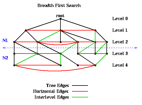
For example, the following figure shows a graph, as well as the embedded BFS tree (edges shown
in black). In addition to the tree edges, there are two other kinds of edges.

The most important fact about the BFS tree is that there are no edges connecting nodes in levels differing by more than 1. In other words, all edges are between nodes in the same level or adjacent levels. The reason is this: Suppose an edge connects n1 and n2 and that (without loss of generality) n1 is visited first by the algorithm. Then the level of n2 is at least as large as the level of n1. The level of n2 can be at most one higher than the level of n1, because it will be visited as a child of n2.
This fact means that simply partitioning the graph into nodes at level L or lower, and nodes at level L+1 or higher, guarantees that only tree and interlevel edges will be cut. There can be no "extra" edges connecting, say, the root to the leaves of the tree. This is illustrated in the above figure, where the 10 nodes above the dotted blue line are assigned to partition N1, and the 10 nodes below the line as assigned to N2.
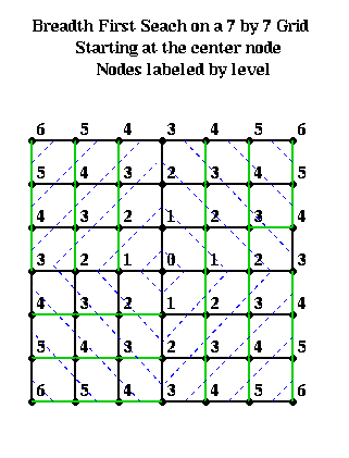
For example, suppose one had an n-by-n mesh with unit distance between nodes. Choose any node r as root from which to build a BFS tree. Then the nodes at level L and above approximately form a diamond centered at r with a diagonal of length 2*L. This is shown below, where nodes are visited counterclockwise starting with the north.

We start with an edge weighted graph G=(N,E,W_E), and a partitioning G = A U B into equal parts: |A| = |B|. Let w(e) = w(i,j) be the weight of edge e=(i,j), where the weight is 0 if no edge e=(i,j) exists. The goal is to find equal-sized subsets X in A and Y in B, such that exchanging X and Y reduces the total cost of edges from A to B. More precisely, we let
T = sum_{a in A and b in B) w(a,b) = cost of edges from A to B
and seek X and Y such that
new_A = A - X U Y and new_B = B - Y U Xhas a lower cost new_T. To compute new_T efficiently, we introduce
  E(a) = external cost of a = sum_{b in B} w(a,b)
  I(a) = internal cost of a = sum_{a' in A, a' != a} w(a,a')
  D(a) = cost of a = E(a) - I(a)
and analogously
  E(b) = external cost of b = sum_{a in A} w(a,b)
  I(b) = internal cost of b = sum_{b' in B, b' != b} w(b,b')
  D(b) = cost of b = E(b) - I(b)
Then it is easy to show that swapping a in A and b in B changes T to
  new_T = T - ( D(a) + D(b) - 2*w(a,b) )
        = T - gain(a,b)
In other words, gain(a,b) = D(a)+D(b)-2*w(a,b) measures the improvement in the
partitioning by swapping a and b.
D(a') and D(b') also change to
  new_D(a') = D(a') + 2*w(a',a) - 2*w(a',b)     for all a' in A, a' != a
  new_D(b') = D(b') + 2*w(b',b) - 2*w(b',a)     for all b' in B, b' != b
Now we can state the Kernighan/Lin algorithm
(0)   Compute T = cost of partition N = A U B                     ... cost = O(|N|^2)
      Repeat
(1)       Compute costs D(n) for all n in N                       ... cost = O(|N|^2)
(2)       Unmark all nodes in G                                   ... cost = O(|N|)
(3)       While there are unmarked nodes                          ... |N|/2 iterations
(3.1)         Find an unmarked pair (a,b) maximizing gain(a,b)    ... cost = O(|N|^2)
(3.2)         Mark a and b (but do not swap them)                 ... cost = O(1)
(3.3)         Update D(n) for all unmarked n, as though a and b
                   had been swapped                               ... cost = O(|N|)
         End while
         ... At this point, we have computed a sequence of pairs
         ...     (a1,b1), ... , (ak,bk) and gains gain(1), ..., gain(k)
         ... where k = |N|/2, ordered by the order in which we marked them
(4)      Pick j maximizing Gain = sum_{i=1}^j gain(i)
         ... Gain is the reduction in cost from swapping (a1,b1),...,(aj,bj)
(5)      If Gain > 0 then
(5.2)         Update A = A - {a1,...,ak} U {b1,...,bk}            ... cost = O(|N|)
(5.2)         Update B = B - {b1,...,bk} U {a1,...,ak}            ... cost = O(|N|)
(5.3)         Update T = T - Gain                                 ... cost = O(1)
         End if
     Until Gain <= 0
In one pass through the Repeat loop, this algorithm computes |N|/2 possible pairs of sets A and B to swap, A = (a1,...,aj) and B=(b1,...,bj), for j=1 to |N|/2. These sets are chosen greedily, so swapping ai and bi makes the most progress of swapping any single pair of nodes. The best of these |N|/2 pairs of sets is chosen, by maximizing Gain. Note that some gains may be negative, if no improvement can be made by swapping just two nodes. Nevertheless, later gains may be large, and so the algorithms can escape this "local minimum".
The cost of each step is shown to the right of the algorithm. Since loop (3) is repeated O(|N|) times, the cost of one pass through the Repeat loop is O(|N|^3). The number of passes through the Repeat loop is hard to predict. Empirical testing by Kernighan and Lin on small graphs (|N|<=360), showed convergence after 2 to 4 passes. For a random graph, the probability of getting the optimum in one pass appears to shrink like 2^(|N|/30). A parallel implementation of this algorithm was design by J. Gilbert and E. Zmijewski in 1987.