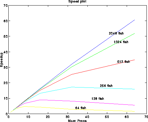
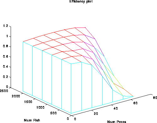
Efficiency is defined as Efficiency(p) = Speedup(p)/p. So, p-linear speedup corresponds to constant efficiency. Our goal is to write algorithms where the efficiency (correspondingly speedup) is as large as possible for every p.
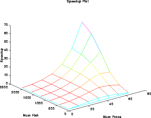
There are essentially two ways to plot Speedup and efficiency, both are easily done in matlab with this code. The first way is to use multiple overlayed 2D plots. This method is best when you wish to obtain actual numbers (i.e., find the speedup for 32 processors, say).


The second way uses a surface plot. This method is less quantitative, but shows the overall trends a bit better.
In general, this method for computing speedup is called "Constant
problem size" scaling. That is, the problem size remains fixed as we
increase the number of processors. Supposing that a program is
composed of an inherently serial portion and a parallelizable portion
(with relative proportions being s and f respectively), the speedup
with n processors becomes Speedup(p) = T(1)/(T(1)s + T(1)f/p) =
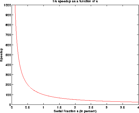
1/(s+f/p) which is necessarily less than 1/s. So, the speedup is
bounded by 1/s. Suppose that s is 5 percent, then 1/s = 20, and it
does not portend well to use more than a 20 processor machine.
In fact, it doesn't look like MPP machines with O(1000) processors
could be useful (refuted
here).
This was the Amdahl argument.
The following plot shows speedup under Amdahl's law.
This was the state of affairs until Gustafson's short but sweet paper [GUS1]. In it, he claimed that these speedup assumptions were unrealistic because the problem size almost never stays fixed while the number of processors grows. Either we'll want to solve a larger problem (e.g., more particles), or solve the problem more accurately (e.g., more grid cells, smaller time step, etc.). In either case, s and f change as the number of processors grows.
Gustafson claimed that it was more realistic to take on a parallel-centric point of view, where we view s and f, the serial and parallel fractional running times, from the point of view of the parallel processor. So, the relative serial time would therefore be s + p*f, and the speedup becomes Speedup(p) = (s+p*f)/(s+p) = p + (1-p)*s, a decreasing line. The key assumption here is that the parallel portion of the program scales linearly with the number of processors. This was the first definition of scaled speedup.
A similar measure of scaled speedup was given in class, i.e., that scaled speedup is given as T(1,n(p))/T(p,n(p)) and scaled efficiency given as T(1,n(p))/(T(p,n(p))*p), where n(p) gives the problem size as a function of the number of processors. Typically, we'll take n(p) to be a linear function of p, i.e., n(p) = a*p, where a is a constant factor.
There are two potential problem with this approach. If n(p) is too large to run on one or a few processors, T(1,n(p)) is not computable. The solution, of course, is to base things not on single processor performance but on multi processor performance, so the speedup becomes T(min_p,n(p))/T(p,n(p)) where min_p is the minimum number of processors that can handle a job of size n(p).
The second problem is perhaps more severe. If the time complexity of the problem grows, say, quadratically with the problem size, then it is possible that the execution time on many processors will be unacceptably large. For example, suppose an algorithm takes time O(n^2) for data size O(n). If n(p) = a*p, then the time for 1 processor will be O((n(1))^2) = O(a^2), whereas the time for p processors, under an ideal linear speedup, will be O((n(p))^2)/p = O(a^2 p^2)/p = O(a^2 * p), a factor of p longer. So even under ideal speedup conditions, the parallel time will increase linearly with the number of processors. The solution is to 1) use a very small 'a', 2) do not increase p very much, or (best but hardest) 3) change the algorithm and reduce the quadratic time complexity.
You'll find that these problems become particularly severe when you and the rest of the class are running code on the cm5 the night before a problem set is due, and the memory and time constraints are even more severe. For plotting, both problems can be addressed by skipping certain data points (the ones you can't run for some reason) in the execution time matrix. In matlab, we can do this by filling in those data points with NaN, the IEEE not a number. Fortunately, matlab's plotting facilities will treat those entries as if they were not there. See here for a matlab plotting example that uses NaNs.
Another type of speedup is to use "Time-constrained scaling", where the absolute wall-clock time is held fixed as more processors are added. In this case, speedup is defined as Speedup(p) = Work(p)/Work(1) where Work(p) is the amount of "work" (defined in an application dependent way) that is done by p processors in a fixed amount of time.
Alas, we have problems here as well because the problem size might be limited regardless of the number of processors available. One reason is that the "concurrency" (i.e., how much there is to do in parallel) often scales at most linearly with n, the problem size. If the concurrency is C, when we can usefully use only C processors. If the number of processors required to keep the running time fixed grows quadratically with the problem size, but the concurrency is linear, we will eventually reach a point where the required number of processors exceeds the concurrency. Then, we'll be forced to stop.
A final type of speedup usable only for scientific applications is error-based scaling. Here, all parameters that control the error of the algorithm are scaled with increasing processors in such a way that the error contribution from each parameter is about the same. The interested reader should consult [SHG] for more information.
The bottom line? The quantitative display of speedup and efficiency is still a pseudo-science. You should concentrate most on displaying the information you've obtained as accurately, clearly, and as simply as possible. Also, use the plotting techniques demonstrated above.
References:
[GUS1] Re-evaluating amdahl's law. John L. Gustafson.
CACM(31)5 May 1988.
[SHG] Scaling Parallel Programs for Multiprocessors:
Methodology and Examples: J.P. Singh, J.L. Hennessy.,
and A. Gupta. IEEE Computer, July 1993.