Optometry and Vision Science article
Gaussian Power with Cylinder Vector Field Representation for Corneal Topography Maps

Overview

This is our paper "Gaussian Power with Cylinder Vector Field Representation for Corneal Topography Maps" published in Optometry and Vision Science, Vol. 74, No. 11, Nov. 1997, pp. 917-925.

The Paper

"Gaussian Power with Cylinder Vector Field Representation for Corneal Topography Maps"* (65Kb postscript file) *Note: This is a slightly earlier version of the paper than the one that actually appeared in the journal.

The Figures

	Figure 1
	A meridional plane, depicted as an orange plane. This plane contains the corneal point of interest (shown as a green dot) and the videokeratograph axis (depicted as a red vector).
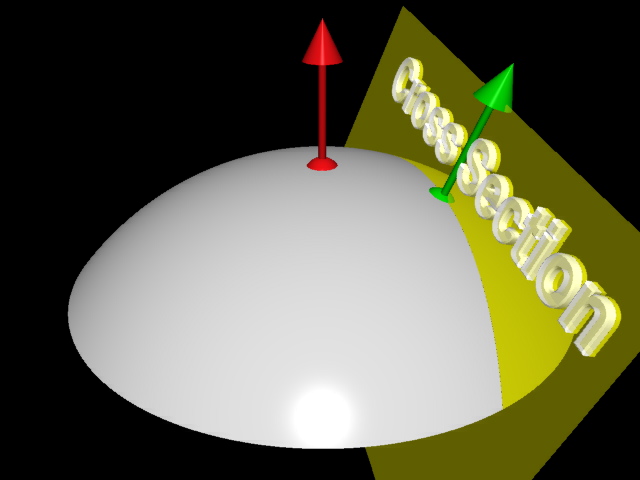
	Figure 2
	The yellow cross-sectional plane contains the normal vector at the point of interest (shown as a green dot). This diagram differs from the one published in that this one has a green vector through the point of interest to indicate the surface normal at that point.
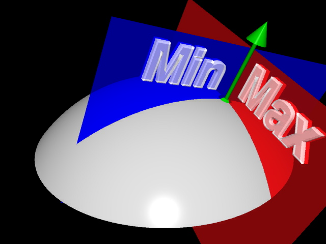
	Figure 3
	Ths planes corresponding to the minimum and maximum curvature directions are shown in blue and red, respectively. This diagram differs from the one published in that this one has a green vector through the point of interest to indicate the surface normal at that point.
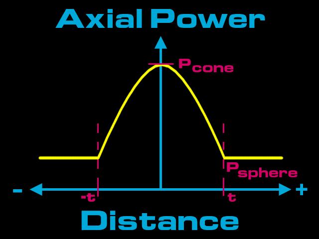
	Figure 4
	This graph illustrates the base corneal model without keratoconus. The model is a simple sphere with constant axial power across its surface. This is represented here as a yellow straight line when plotting axial power vs. diatance. The power is denoted P_sphere, and is labeled in red.
	Figure 5
	To model keratoconus, a section of the sphere is removed and replaced with a surface of revolution formed from a hyperbola. The axial power associated with the hyperbola between -t and t is shown as the yellow curve. The maximum power of the cone is denoted P_cone.
	Figure 6(i)
	This shows a mock-up, depicting in each figure component 6(i) thorugh 6(v), the center of the simulated cone (middle), instantaneous power (upper left), axial power (upper right), Gaussian power with a cylinder overlay (lower left), and the height map, or radial difference from the reference sphere (lower right). The center of the cone is at phi = 12° and theta = 215°. Here P_cone = P_sphere = 45 D; thus, there is no keratoconus and all power maps are constant.
	Figure 6(ii)
	Same as Fig. 6(i), except P_cone is set to 57 D of axial power, slightly larger than P_sphere. The cone is shown in green in the model.
	Figure 6(iii)
	The parameter P_cone has now reached its maximum value of 82 D.
	Figure 6(iv)
	The parameter P_cone is fixed at 82 D and the cone is rotated toward the center of the cornea. Its center is now at phi = 6°.
	Figure 6(v)
	The center of the cone is now at phi = 0° (directly at the north pole).
	Figure 7
	The four views of regular fixation (patient looking directly into the center of the videokeratograph): instantaneous power (upper left), axial power (upper right), Gaussian power with a cylinder overlay (lower left), and the radial difference from a reference sphere (lower right).
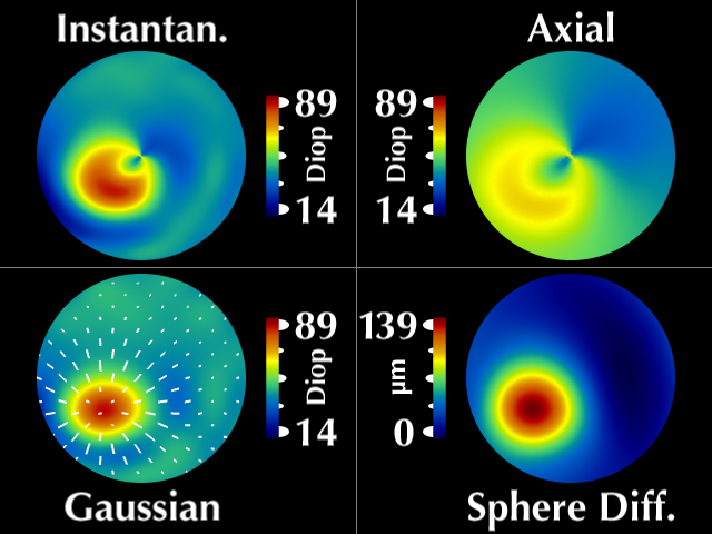
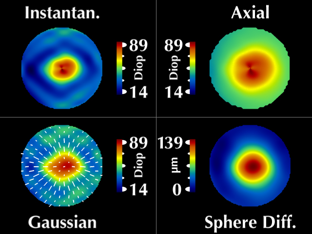
	Figure 8
	The four views of conic alignment (patient shifting his gaze direction up toward his left so that the cone alights with the center of the videokeratograph): instantaneous power (upper left), axial power (upper right), Gaussian power with a cylinder overlay (lower left), and the radial difference from a reference sphere (lower right).