CS 189/289A Introduction to Machine Learning Jonathan Shewchuk Spring 2024 Mondays and Wednesdays, 6:30–8:00 pm Wheeler Hall Auditorium (a.k.a. 150 Wheeler Hall) Begins Wednesday, January 17 Discussion sections begin Tuesday, January 23 Contact: Use Ed Discussion for public and private questions that can be viewed by all the TAs. I check Ed Discussion far more often and reliably than email. For very personal issues, send email to jrs@berkeley.edu. My office hours: Mondays, 5:10–6:00 pm Fridays, 5:10–6:00 pm and by appointment. (I'm usually free after the lectures too.)

This class introduces algorithms for learning, which constitute an important part of artificial intelligence.

Topics include

• classification: perceptrons, support vector machines (SVMs), Gaussian discriminant analysis (including linear discriminant analysis, LDA, and quadratic discriminant analysis, QDA), logistic regression, decision trees, neural networks, convolutional neural networks, boosting, nearest neighbor search;
• regression: least-squares linear regression, logistic regression, polynomial regression, ridge regression, Lasso;
• density estimation: maximum likelihood estimation (MLE);
• dimensionality reduction: principal components analysis (PCA), random projection; and
• clustering: k-means clustering, hierarchical clustering.

Useful Links

• Access the CS 189/289A Ed Discussion forum. If you haven't already been added to the class, use this invitation link.
• Submit your assignments at the CS 189/289A Gradescope. If you need the entry code, find it on Ed Discussion in the post entitled “Welcome to CS 189!”
• If you want an instructional account, you can get one online. Go to the same link if you forget your password or account name.
• Check out this Machine Learning Visualizer by our former TA Sagnik Bhattacharya and his teammates Colin Zhou, Komila Khamidova, and Aaron Sun. It's a great way to build intuition for what decision boundaries different classification algorithms find.

Prerequisites

• Math 53 (or another vector calculus course),
• Math 54, Math 110, or EE 16A+16B (or another linear algebra course),
• CS 70, EECS 126, or Stat 134 (or another probability course).
• Enough programming experience to be able to debug complicated programs without much help. (Unlike in a lower-division programming course, the Teaching Assistants are under no obligation to look at your code.)

If you want to brush up on prerequisite material:

• There's a fantastic collection of linear algebra visualizations on YouTube by 3Blue1Brown (Grant Sanderson) starting with this playlist, The Essence of Linear Algebra. I highly recommend them, even if you think you already understand linear algebra. It's not enough to know how to work with matrix algebra equations; it's equally important to have a geometric intuition for what it all means.
• Here's a short summary of math for machine learning written by our former TA Garrett Thomas.
• Stanford's machine learning class provides additional reviews of linear algebra and probability theory.
• To learn matrix calculus (which will rear its head first in Homework 2), check out the first two chapters of The Matrix Cookbook.
• Another locally written review of linear algebra appears in this book by Prof. Laurent El Ghaoui.
• An alternative guide to CS 189 material (if you're looking for a second set of lecture notes besides mine), written by our former TAs Soroush Nasiriany and Garrett Thomas, is available at this link. I recommend reading my notes first, but reading the same material presented a different way can help you firm up your understanding.

Textbooks

Both textbooks for this class are available free online. Hardcover and eTextbook versions are also available.

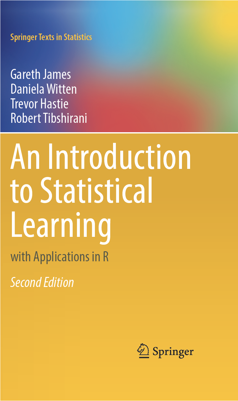
• Gareth James, Daniela Witten, Trevor Hastie, and Robert Tibshirani, An Introduction to Statistical Learning with Applications in R, second edition, Springer, New York, 2021. ISBN # 978-1-0716-1417-4. See Amazon for hardcover or eTextbook.
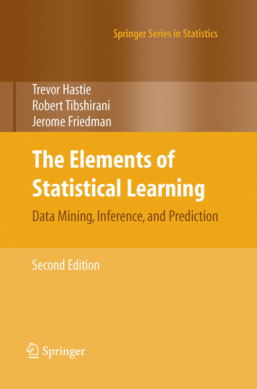
• Trevor Hastie, Robert Tibshirani, and Jerome Friedman, The Elements of Statistical Learning: Data Mining, Inference, and Prediction, second edition, Springer, 2008. See Amazon for hardcover or eTextbook.

Homework and Exams

You have a total of 5 slip days that you can apply to your semester's homework. We will simply not award points for any late homework you submit that would bring your total slip days over five. If you are in the Disabled Students' Program and you are offered an extension, even with your extension plus slip days combined, no single assignment can be extended more than 5 days. (We have to grade them sometime!)

The following homework due dates are tentative and may change.

Homework 1 is due Wednesday, January 24 at 11:59 PM. (Warning: 16 MB zipfile. Here's just the written part.)

Homework 2 is due Wednesday, February 7 at 11:59 PM. (PDF file only.)

Homework 3 is due Friday, February 23 at 11:59 PM. (Warning: 15 MB zipfile. Here's just the written part.)

Homework 4 is due Friday, March 8 at 11:59 PM. (Here's just the written part.)

Homework 5 is due Tuesday, April 2 at 11:59 PM. (Here's just the written part.)

Homework 6 is due Friday, April 19 at 11:59 PM. (Warning: 137 MB zipfile. Here's just the written part.) Important: For Homework 6 only, the “HW6 Code” assignment on Gradescope has an autograder for some parts of the homework. The grade you receive on the coding questions will directly reflect the score reported by the autograder!

Homework 7 is due Wednesday, May 1 at 11:59 PM. (Warning: 116 MB zipfile. Here's just the written part.)

The CS 289A Project has a proposal due Friday, April 12. The video is due Monday, May 6, and the final report is due Tuesday, May 7.

The Midterm took place on Monday, March 11 at 6:30–8:00 PM in multiple rooms on campus. Previous midterms are available: Without solutions: Spring 2013, Spring 2014, Spring 2015, Fall 2015, Spring 2016, Spring 2017, Spring 2019, Summer 2019, Spring 2020 Midterm A, Spring 2020 Midterm B, Spring 2021, Spring 2022, Spring 2023, Spring 2024. With solutions: Spring 2013, Spring 2014, Spring 2015, Fall 2015, Spring 2016, Spring 2017, Spring 2019, Summer 2019, Spring 2020 Midterm A, Spring 2020 Midterm B, Spring 2021, Spring 2022, Spring 2023, Spring 2024.

The Final Exam will take place on Friday, May 10 at 3–6 PM in four different rooms on campus. (Check Ed Discussions for your room.) Previous final exams are available. Without solutions: Spring 2013, Spring 2014, Spring 2015, Fall 2015, Spring 2016, Spring 2017, Spring 2019, Spring 2020, Spring 2021, Spring 2022, Spring 2023. With solutions: Spring 2013, Spring 2014, Spring 2015, Fall 2015, Spring 2016, Spring 2017, Spring 2019, Spring 2020, Spring 2021, Spring 2022, Spring 2023.

Lectures

Lecture 1 (January 17): Introduction. Classification. Training, validation, and testing. Overfitting and underfitting. Read ESL, Chapter 1. My lecture notes (PDF). The lecture video. In case you don't have access to bCourses, here's a backup screencast (screen only).

Lecture 2 (January 22): Linear classifiers. Decision functions and decision boundaries. The centroid method. Perceptrons. Read parts of the Wikipedia Perceptron page. Optional: Read ESL, Section 4.5–4.5.1. My lecture notes (PDF). The lecture video. In case you don't have access to bCourses, here's a backup screencast (screen only).

Lecture 3 (January 24): Gradient descent, stochastic gradient descent, and the perceptron learning algorithm. Feature space versus weight space. The maximum margin classifier, aka hard-margin support vector machine (SVM). Read ISL, Section 9–9.1. My lecture notes (PDF). The lecture video. In case you don't have access to bCourses, here's a backup screencast (screen only).

Lecture 4 (January 29): The support vector classifier, aka soft-margin support vector machine (SVM). Features and nonlinear decision boundaries. Read ESL, Section 12.2 up to and including the first paragraph of 12.2.1. My lecture notes (PDF). The lecture video. In case you don't have access to bCourses, here's a backup screencast (screen only).

Lecture 5 (January 31): Machine learning abstractions: application/data, model, optimization problem, optimization algorithm. Common types of optimization problems: unconstrained, linear programs, quadratic programs. The influence of the step size on gradient descent. Optional: Read (selectively) the Wikipedia page on mathematical optimization. My lecture notes (PDF). The lecture video. In case you don't have access to bCourses, here's a backup screencast (screen only).

Lecture 6 (February 5): Decision theory, also known as risk minimization: the Bayes decision rule and the Bayes risk. Generative and discriminative models. Read ISL, Section 4.4 (the first few pages). My lecture notes (PDF). The lecture video. In case you don't have access to bCourses, here's a backup screencast (screen only).

Lecture 7 (February 7): Gaussian discriminant analysis, including quadratic discriminant analysis (QDA) and linear discriminant analysis (LDA). Maximum likelihood estimation (MLE) of the parameters of a statistical model. Fitting an isotropic Gaussian distribution to sample points. Read ISL, Section 4.4 (all of it). Optional: Read (selectively) the Wikipedia page on maximum likelihood estimation. My lecture notes (PDF). The lecture video. In case you don't have access to bCourses, here's a backup screencast (screen only).

Lecture 8 (February 12): Eigenvectors, eigenvalues, and the eigendecomposition of a symmetric real matrix. The quadratic form and ellipsoidal isosurfaces as an intuitive way of understanding symmetric matrices. Application to anisotropic multivariate normal distributions. The covariance of random variables. Read Chuong Do's notes on the multivariate Gaussian distribution. My lecture notes (PDF). The lecture video. In case you don't have access to bCourses, here's a backup screencast (screen only).

Lecture 9 (February 14): MLE, QDA, and LDA revisited for anisotropic Gaussians. Read ISL, Sections 4.4 and 4.5. My lecture notes (PDF). The lecture video. In case you don't have access to bCourses, here's a backup screencast (screen only).

February 19 is Presidents' Day.

Lecture 10 (February 21): Regression: fitting curves to data. The 3-choice menu of regression function + loss function + cost function. Least-squares linear regression as quadratic minimization. The design matrix, the normal equations, the pseudoinverse, and the hat matrix (projection matrix). Logistic regression; how to compute it with gradient descent or stochastic gradient descent. Read ISL, Sections 4–4.3. My lecture notes (PDF). The lecture video. In case you don't have access to bCourses, here's a backup screencast (screen only).

Lecture 11 (February 26): Newton's method and its application to logistic regression. LDA vs. logistic regression: advantages and disadvantages. ROC curves. Weighted least-squares regression. Least-squares polynomial regression. Read ISL, Sections 7.1, 9.3.3; ESL, Section 4.4.1. Optional: here is a fine short discussion of ROC curves—but skip the incoherent question at the top and jump straight to the answer. My lecture notes (PDF). The lecture video. In case you don't have access to bCourses, here's a backup screencast (screen only).

Lecture 12 (February 28): Statistical justifications for regression. The empirical distribution and empirical risk. How the principle of maximum likelihood motivates the cost functions for least-squares linear regression and logistic regression. The bias-variance decomposition; its relationship to underfitting and overfitting; its application to least-squares linear regression. Read ESL, Sections 2.6 and 2.9. Optional: Read the Wikipedia page on the bias-variance trade-off. My lecture notes (PDF). The lecture video. In case you don't have access to bCourses, here's a backup screencast (screen only).

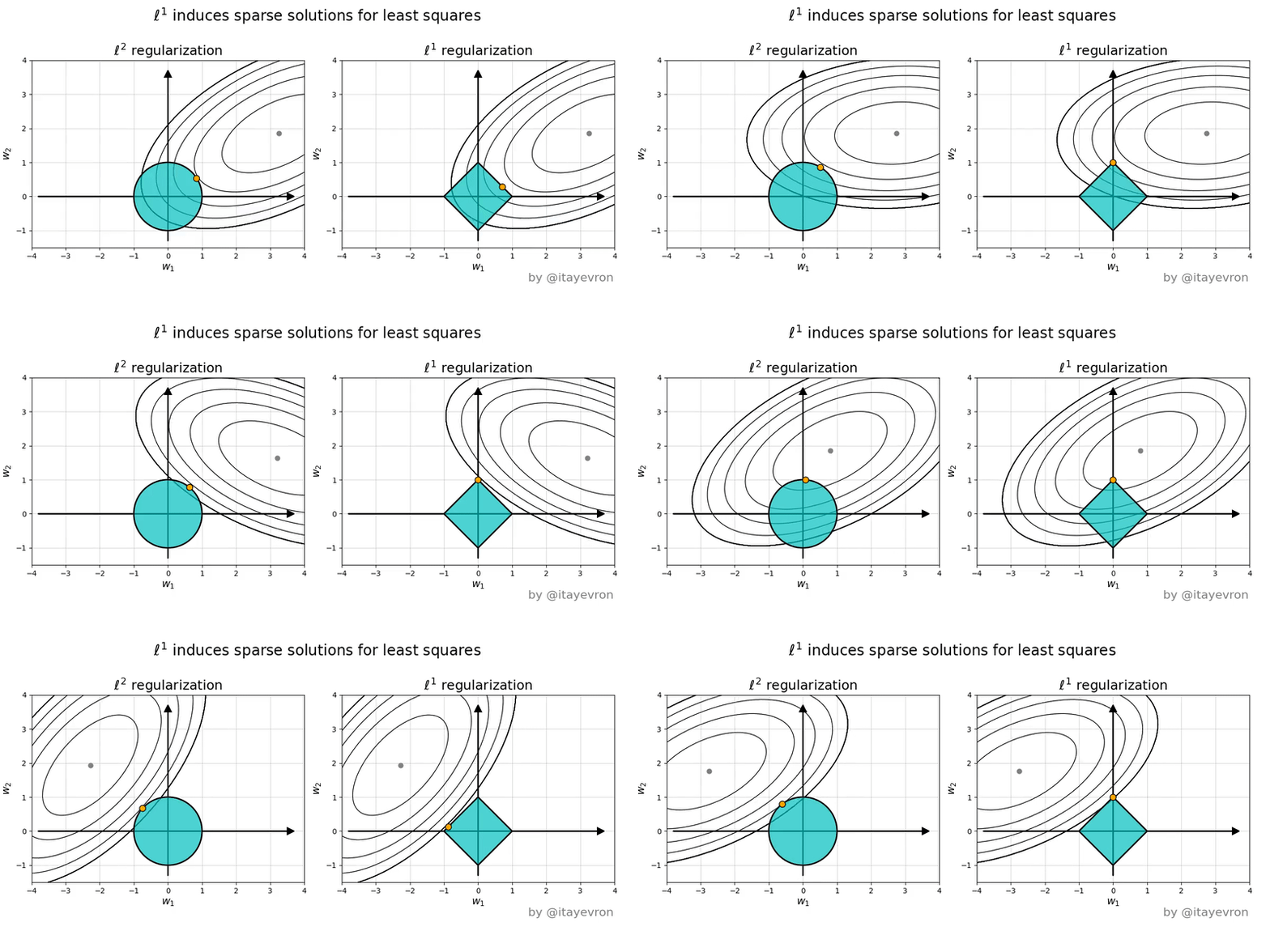
Lecture 13 (March 4): Ridge regression: penalized least-squares regression for reduced overfitting. How the principle of maximum a posteriori (MAP) motivates the penalty term (aka Tikhonov regularization). Subset selection. Lasso: penalized least-squares regression for reduced overfitting and subset selection. Read ISL, Sections 6–6.1.2, the last part of 6.1.3 on validation, and 6.2–6.2.1; and ESL, Sections 3.4–3.4.3. Optional: This CrossValidated page on ridge regression is pretty interesting. My lecture notes (PDF). The lecture video. In case you don't have access to bCourses, here's a backup screencast (screen only).

Lecture 14 (March 6): Decision trees; algorithms for building them. Entropy and information gain. Read ISL, Sections 8–8.1. My lecture notes (PDF). The lecture video. In case you don't have access to bCourses, here's a backup screencast (screen only).

The Midterm took place on Monday, March 11 at 6:30–8:00 PM in multiple rooms on campus. The midterm covers Lectures 1–13, the associated readings listed on the class web page, Homeworks 1–4, and discussion sections related to those topics.

Lecture 15 (March 13): More decision trees: decision tree regression; stopping early; pruning; multivariate splits. Ensemble learning, bagging (bootstrap aggregating), and random forests. Read ISL, Section 8.2. The animations I show in class are available in this directory. My lecture notes (PDF). The lecture video. In case you don't have access to bCourses, here's a backup screencast (screen only).

Lecture 16 (March 18): Kernels. Kernel ridge regression. The polynomial kernel. Kernel perceptrons. Kernel logistic regression. The Gaussian kernel. Optional: Read ISL, Section 9.3.2 and ESL, Sections 12.3–12.3.1 if you're curious about kernel SVM. My lecture notes (PDF). The lecture video. In case you don't have access to bCourses, here's a backup screencast (screen only).

Lecture 17 (March 20): Neural networks. Gradient descent and the backpropagation algorithm. Read ESL, Sections 11.3–11.4. Optional: Welch Labs' video tutorial Neural Networks Demystified on YouTube is quite good (note that they transpose some of the matrices from our representation). Also of special interest is this Javascript neural net demo that runs in your browser. Here's another derivation of backpropagation that some people have found helpful. My lecture notes (PDF). The lecture video. In case you don't have access to bCourses, here's a backup screencast (screen only).

March 25–29 is Spring Recess.

Lecture 18 (April 1): The vanishing gradient problem. Rectified linear units (ReLUs). Backpropagation with softmax outputs and cross-entropy loss. Neuron biology: axons, dendrites, synapses, action potentials. Differences between traditional computational models and neuronal computational models. Optional: Try out some of the Javascript demos on this excellent web page—and if time permits, read the text too. The first four demos illustrate the neuron saturation problem and its fix with the logistic loss (cross-entropy) functions. The fifth demo gives you sliders so you can understand how softmax works. My lecture notes (PDF). Note: the material on neurobiology in the Lecture 18 notes was not covered by Prof. Sahai, so it is not in scope for the Final Exam. Prof. Anant Sahai's lecture video. In case you don't have access to bCourses, here's a backup screencast (screen only).

Lecture 19 (April 3): Heuristics for faster training. Heuristics for avoiding bad local minima. Heuristics to avoid overfitting. Convolutional neural networks. Neurology of retinal ganglion cells in the eye and simple and complex cells in the V1 visual cortex. Read ESL, Sections 11.5 and 11.7. Here is the video about Hubel and Wiesel's experiments on the feline V1 visual cortex. Here is Yann LeCun's video demonstrating LeNet5. Optional: A fine paper on heuristics for better neural network learning is Yann LeCun, Leon Bottou, Genevieve B. Orr, and Klaus-Robert Müller, “Efficient BackProp,” in G. Orr and K.-R. Müller (Eds.), Neural Networks: Tricks of the Trade, Springer, 1998. Also of special interest is this Javascript convolutional neural net demo that runs in your browser. Some slides about the V1 visual cortex and ConvNets (PDF). My lecture notes (PDF). Note: the material on the visual cortex in the Lecture 19 notes was not covered by Prof. Sahai, so it is not in scope for the Final Exam. Prof. Anant Sahai's lecture video. In case you don't have access to bCourses, here's a backup screencast (screen only).

Lecture 20 (April 8): Unsupervised learning. Principal components analysis (PCA). Derivations from maximum likelihood estimation, maximizing the variance, and minimizing the sum of squared projection errors. Eigenfaces for face recognition. Read ISL, Sections 12–12.2 (if you have the first edition, Sections 10–10.2) and the Wikipedia page on Eigenface. Optional: Watch the video for Volker Blanz and Thomas Vetter's A Morphable Model for the Synthesis of 3D Faces. My lecture notes (PDF). The lecture video. In case you don't have access to bCourses, here's a backup screencast (screen only).

Lecture 21 (April 10): The singular value decomposition (SVD) and its application to PCA. Clustering: k-means clustering aka Lloyd's algorithm; k-medoids clustering; hierarchical clustering; greedy agglomerative clustering. Dendrograms. Read ISL, Section 12.4 (if you have the first edition, Section 10.3). My lecture notes (PDF). The lecture video. In case you don't have access to bCourses, here's a backup screencast (screen only).

Lecture 22 (April 15): The geometry of high-dimensional spaces. Random projection. The pseudoinverse and its relationship to the singular value decomposition. Optional: Mark Khoury, Counterintuitive Properties of High Dimensional Space. Optional: The Wikipedia page on the Moore–Penrose inverse. For reference: Sanjoy Dasgupta and Anupam Gupta, An Elementary Proof of a Theorem of Johnson and Lindenstrauss, Random Structures and Algorithms 22(1)60–65, January 2003. My lecture notes (PDF). The lecture video. In case you don't have access to bCourses, here's a backup screencast (screen only).

Lecture 23 (April 17): Learning theory. Range spaces (aka set systems) and dichotomies. The shatter function and the Vapnik–Chervonenkis dimension. Read Andrew Ng's CS 229 lecture notes on learning theory. For reference: Thomas M. Cover, Geometrical and Statistical Properties of Systems of Linear Inequalities with Applications in Pattern Recognition, IEEE Transactions on Electronic Computers 14(3):326–334, June 1965. My lecture notes (PDF). The lecture video. In case you don't have access to bCourses, here's a backup screencast (screen only).

Lecture 24 (April 22): AdaBoost, a boosting method for ensemble learning. Nearest neighbor classification and its relationship to the Bayes risk. Read ESL, Sections 10–10.5, and ISL, Section 2.2.3. For reference: Yoav Freund and Robert E. Schapire, A Decision-Theoretic Generalization of On-Line Learning and an Application to Boosting, Journal of Computer and System Sciences 55(1):119–139, August 1997. Freund and Schapire's Gödel Prize citation and their ACM Paris Kanellakis Theory and Practice Award citation. For reference: Thomas M. Cover and Peter E. Hart, Nearest Neighbor Pattern Classification, IEEE Transactions on Information Theory 13(1):21–27, January 1967. For reference: Evelyn Fix and J. L. Hodges Jr., Discriminatory Analysis---Nonparametric Discrimination: Consistency Properties, Report Number 4, Project Number 21-49-004, US Air Force School of Aviation Medicine, Randolph Field, Texas, 1951. See also This commentary on the Fix–Hodges paper.

Lecture 25 (April 24): The exhaustive algorithm for k-nearest neighbor queries. Speeding up nearest neighbor queries. Voronoi diagrams and point location. k-d trees. Application of nearest neighbor search to the problem of geolocalization: given a query photograph, determine where in the world it was taken. If I like machine learning, what other classes should I take? For reference: the best paper I know about how to implement a k-d tree is Sunil Arya and David M. Mount, Algorithms for Fast Vector Quantization, Data Compression Conference, pages 381–390, March 1993. For reference: the IM2GPS web page, which includes a link to the paper.

The Final Exam will take place on Friday, May 10, 3–6 PM.

Discussion Sections and Teaching Assistants

Sections begin to meet on January 23.

Your Teaching Assistants are:
Suchir Agarwal
Samuel Alber
Pierre Boyeau
Charles Dove
Lydia Ignatova
Aryan Jain
Ziye Ma
Norman Mu
Andrew Qin
Sowmya Thanvantri
Kevin Wang
Zekai Wang
Richard Wu
Gavin Zhang

Grading

• 40% for homeworks.
• 20% for the Midterm.
• CS 189: 40% for the Final Exam.
• CS 289A: 20% for the Final Exam.
• CS 289A: 20% for a Project.

Supported in part by the National Science Foundation under Awards CCF-0430065, CCF-0635381, IIS-0915462, CCF-1423560, and CCF-1909204, in part by a gift from the Okawa Foundation, and in part by an Alfred P. Sloan Research Fellowship.

Copyright 2023 by Jason Diwa