GPCA: Basic Ideas via a Simple Example
GPCA algorithms all have an
algebraic underpinning. This page will introduce you to some
of the fundamental concepts via some simple examples. We assume that you are
already familiar with the type of problems GPCA is trying to solve.
If not, you may want to skim through the
Introduction section.
Two Lines in a Plane
Let us first consider the simplest
data set, namely two lines inside a plane. Note that since these are
one-dimensional subspaces in a plane.
Since they are of one dimension less than the ambient
space (i.e. codimension one), we will refer to them as hyperplanes.
Hyperplanes have a very nice algebraic property. Since a hyperplane is of codimension one by definition, it can be parameterized by a single vector, namely the normal vector that is orthogonal to it. The following images show the coordinate axes for R2 (dashed black lines), some data samples from two lines S1 and S2 (colored dots), and the vectors b1 and b2 normal to the subspaces (arrows of corresponding color).
Hyperplanes have a very nice algebraic property. Since a hyperplane is of codimension one by definition, it can be parameterized by a single vector, namely the normal vector that is orthogonal to it. The following images show the coordinate axes for R2 (dashed black lines), some data samples from two lines S1 and S2 (colored dots), and the vectors b1 and b2 normal to the subspaces (arrows of corresponding color).

Since every data sample x = [x y]T in S1 is orthogonal to b1, we have that :

and similarly for a point in S2,
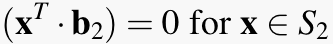
Since we know that any point in the data set must belong to either S1 or S2, we then have that:

Since we know that any point in the data set must belong to either S1 or S2, we then have that:
Then the key idea of GPCA is to directly find the polynomials that fit all the data points simultaneously. In the above example, it first identifies the quadratic polynomial that fits the two lines. Then the derivative of the polynomial evaluated at any point x on the first line is proportional to b1; and the derivative evaluated at any point x on the second line is proportional to b2. In this way, we can retrieve the model of the two lines from such fitting polynomials.
Many of the ideas can be generalized to an arbitrary number of subspaces of arbitrary dimensions. One can find a complete and general theory of GPCA in the literature listed in the Publications section.