


Next: Finding
correspondences Up: A
radial cumulative similarity Previous: Introduction
A robust image transform
Since contrast determines the ability to find unique correspondences, we
motivate our approach by considering the sources of contrast within a local
image window that contains an occlusion boundary. We define the ``foreground''
to be the scene layer on which the central point of the window resides;
points on all other layers are considered ``background''. We desire a transform
which ignores background contrast but is sensitive to contrast energy from
the occluding boundaries of the foreground layer.
In general one does not know a priori whether contrast within
a particular window is entirely within the foreground layer, is due to
the occlusion boundary between foreground and background, or is entirely
within the background layer. When contrast is in the foreground layer,
an ideal template would model it fully, both in magnitude and sign. When
the contrast is due to an occlusion edge, it is reasonable only to define
a template based on the contrast energy, since the sign of contrast is
arbitrary with changing background. When contrast is in the background
layer, it should be ignored in an ideal template.
Figure 3: Construction of
the Radial Cumulative Similarity (RCS) transform. (a) Color window, (b)
central color  (in box at lower-left) and map of local similarity S. Bright pixels
indicate similar value as central color. (c) neighborhood of cumulative
similarity, N, where each pixel reflects the likelihood the ray
from the center point has uniform color.
(in box at lower-left) and map of local similarity S. Bright pixels
indicate similar value as central color. (c) neighborhood of cumulative
similarity, N, where each pixel reflects the likelihood the ray
from the center point has uniform color.
(a)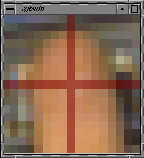 (b) (b)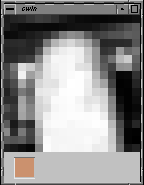 (c) (c)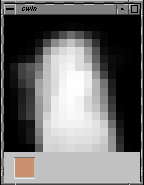 |
We define a robust local image representation that approximates this ideal,
without any prior knowledge of the occlusion location. Our representation
is comprised of a central image-attribute value (typically color) and of
a local contrast neighborhood of this attribute, attenuated to discount
background influence. Many different diffusion functions could be used
to attenuate background influence; in this paper we explore radial cumulative
probability functions. The local neighborhood is defined by estimating
the contrast energy of the attribute relative to the center value, interpreting
this energy probabilistically, and computing the cumulative likelihood
that the attribute is unchanged along the ray from the template center
to a particular neighborhood point.
Formally, given a discrete color image intensity function  we
compute a local robust representation:
we
compute a local robust representation:
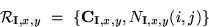 where
where  .
Our representation is comprised of two terms, a central value and a neighborhood
function; the central value is simply the image attribute averaged over
the center point or a small central area:
.
Our representation is comprised of two terms, a central value and a neighborhood
function; the central value is simply the image attribute averaged over
the center point or a small central area:
 where
where  is an image attribute function and can be defined to be any local image
property. In this paper we explore attribute functions which return the
color or hue vector corresponding to the pixel at the given location. We
typically keep the central region small, with Mc = 0
or 1. The neighborhood is defined over window coordinates
using the similarity of other image attribute values to the central value:
is an image attribute function and can be defined to be any local image
property. In this paper we explore attribute functions which return the
color or hue vector corresponding to the pixel at the given location. We
typically keep the central region small, with Mc = 0
or 1. The neighborhood is defined over window coordinates
using the similarity of other image attribute values to the central value:
 Note that
  is a local contrast energy function, and is thus independent of contrast
sign.
is a local contrast energy function, and is thus independent of contrast
sign.
When tracking a single feature of known size, we could simply use  over a fixed (possibly non-rectangular) window cropped to resolve the entire
feature and the occlusion boundary. This would yield a template which captures
both the foreground and occlusion contrast, and was insensitive to contrast
sign. However, when automatically tracking features for image analysis/synthesis,
or when computing dense correspondence for stereo or motion, we rarely
have the luxury of knowledge of appropriate window size.
over a fixed (possibly non-rectangular) window cropped to resolve the entire
feature and the occlusion boundary. This would yield a template which captures
both the foreground and occlusion contrast, and was insensitive to contrast
sign. However, when automatically tracking features for image analysis/synthesis,
or when computing dense correspondence for stereo or motion, we rarely
have the luxury of knowledge of appropriate window size.
For fully automatic processing, we define a function which substantially
attenuates the influence of exterior pixels. We define our neighborhood
function by propagating the attribute similarity function S outward
along a ray from the center of the window, so that once we encounter a
dissimilarity (i.e., contrast energy) we attenuate the influence of any
contrast found farther out along that ray. We are essentially making the
assumption that the most proximate contrast is due either to surface contrast
or occlusion contrast; background contrast must lie beyond an occurrence
of occlusion contrast. Our algorithm reflects the conservative assumption
that, in the absence of any prior knowledge of occlusion location, correspondence
judgments are best made on the most proximate contrast.
Our neighborhood function is the cumulative product of S, computed
radially from the center point:
 where
where  is the set of points that lie along the ray from (0,0) to (i,j),
inclusive. Other possible neighborhood functions include pixel-fill or
diffusion operators; these would also capture non-convex local similarity
structure.
is the set of points that lie along the ray from (0,0) to (i,j),
inclusive. Other possible neighborhood functions include pixel-fill or
diffusion operators; these would also capture non-convex local similarity
structure.
We call the representation  the Radial Cumulative Similarity (RCS) transform, since it reflects
the radial homogeneity of a given attribute value. Figure 3
illustrates the computation of color RCS for a image window containing
a fingertip. The substantial benefit of the RCS transform is invariance
to sign of contrast at an occluding boundary, as well as invariance to
background contrast. As an example Figure 4
shows the RCS transform for the marked locations in Figure 2;
despite dissimilar background structure and occlusion contrast sign reversal,
the transformed pairs are substantially similar.
the Radial Cumulative Similarity (RCS) transform, since it reflects
the radial homogeneity of a given attribute value. Figure 3
illustrates the computation of color RCS for a image window containing
a fingertip. The substantial benefit of the RCS transform is invariance
to sign of contrast at an occluding boundary, as well as invariance to
background contrast. As an example Figure 4
shows the RCS transform for the marked locations in Figure 2;
despite dissimilar background structure and occlusion contrast sign reversal,
the transformed pairs are substantially similar.
Figure 4: The RCS transform is stable
despite occlusion boundaries of different contrast sign. (a,b) show the
RCS transform of the marked locations in Figure 2(b,f),
while (c,d) show the RCS transform of Figure 2(d,h).
(a)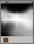 (b) (b)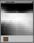 (c) (c)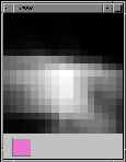 (d) (d)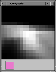 |
Next: Finding
correspondences Up: A
radial cumulative similarity Previous: Introduction
Trevor Darrell
9/9/1998