CS 184: COMPUTER GRAPHICS

PREVIOUS < - - - - > CS 184 HOME < - - - - > CURRENT < - - - - > NEXT

Lecture #12 -- Wed 3/2/2011.

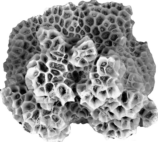
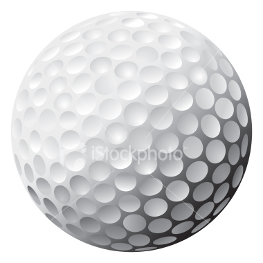
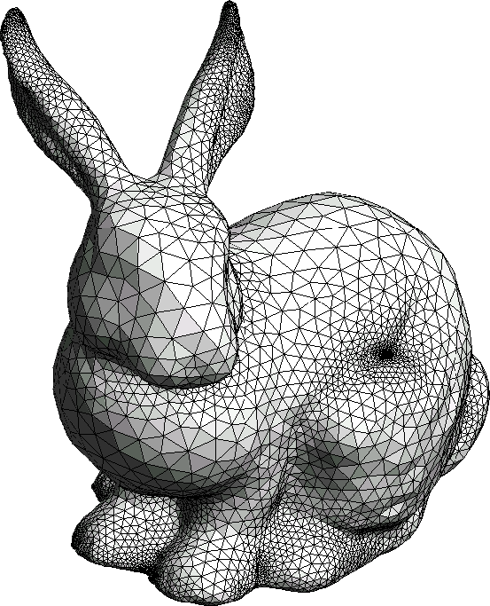
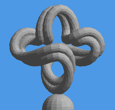
What computer graphics paradigm would you use to model the following items:


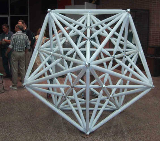
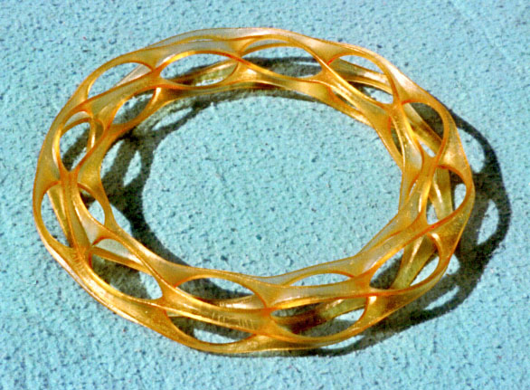
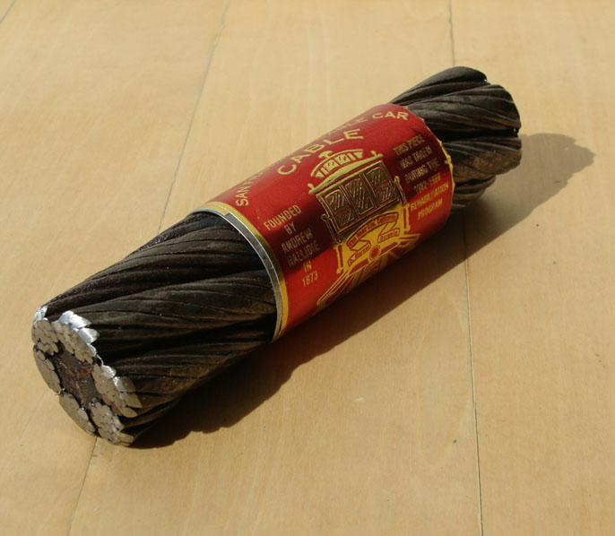
corals	golfball	bunny	sculpture	construction	cable

Various Modeling Paradigms for 3D Objects:

Voxels and Octree:
Concept: sample space regularly;
determine whether the sample falls inside or outside of object, e.g., by an implicit function;
"turn on" inside voxels.
Efficient encoding required: e.g., quadtree in 2D, octree in 3D.
Good for representing: MRI-scans, CAT-scans, brains, sponge-like objects, clouds, ...

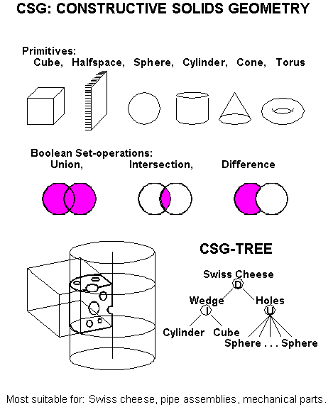
CSG and Boolean set operations:
CSG = Constructive Solid Geometry.
The object is composed from (overlaping) primitive geometric shapes,
typically: cubes, halfspaces, spheres, cylinders, cones, tori, ...
e.g., a "Sausage" = bent cylinder plus spherical end-caps (show 2D composite).
Good for representing: mechanical parts, Swiss cheese, results of solid modeling operations, ...

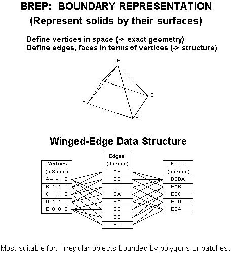
B-rep and winged-edge data structure: [13.1-13.2].

Tessallate surface; describe polyhedral objects via vertices, edges, faces;
or "meshes" (triangle strips, fans) that use a more efficient encoding of the connectivity.
Good for representing: polyhedral objects with odd angles, tessellated parametric surfaces, ...

Procedural modeling:
A program fragment creates the vertices and faces and their connectivity,
or, alternatively, the instance calls to CSG primitives,
or a collection of "inside" voxels,
or an implicit function, which may then be converted to one of the above representations.
Good for representing: parameterized, iterated objects;
e.g., gearwheels, fractal mountains, trees, geometrical sculpture, ...

Commonly used generic procedures: Sweeps: (axial, rotational, or along an arbitrary path).
For "Sausage": Sweep a circle through space along a curve. Start small for front-cap;
keep constant through main part of sausage; taper down to zero for end cap.
Good for representing: pipes, sausages, moldings, rotationally symmetrical (turned) objects, geometrical sculpture, ...

Another example: Subdivision Surfaces (discussed later in the course).

A note on planar faces:

Often you may encounter B-reps with faces that are polygons with four or more faces.
Sometimes not all the vertices of such a face lie in a plane.
Then how do you calculate a plane equation, whichy is needed in the calculation of the illumination:
==> Martin Newell's plane equation formula:
The components of the desired normal vector are in same ratio as the shadows areas of the polygon on the three coord planes.
==> Each shadow area is computed in a 2D projection as a sum of trapezoids (x1-x2)(y1+y2)/2.
==> Form the sum of all such expressions around the contour; do it for all 3 projections.

CS 184 Hall of Fame:

Some special accomplishments in Assignment#5:
Brandon Wang
Kevin Lee
Jennifer To
Jeremy Williams
Jordy Rose

POLL: Does anyone need / is available for partnering for Assignment #6 ?

Introduction to Splines

What are "splines" ? -- Wood strips used in ship building that yield nice smooth curves,
because nature is trying to minimize overall bending energy (= arc-length integral of curvature squared).
Depending on what fixtures are being used one can apply different constraints to those strips:
-- Position Constraints are implemented with pegs, and
-- Tangent Constriants can be realized with clamps.
Most "mathematical splines" used in CG are linearized approximations to the above difficult optimization problem.

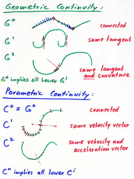
When making smooth shapes by piecing together smooth curves, consider the
degrees of smoothness at the joints:
-- Parametric Continuity: differentiability of the parametric representation (C0, C1, C2, ...)
-- Geometric Continuity: smoothness of the resulting displayed shape (G0=C0, G1=tangent-cont., G2=curvature-cont. )

Distinguish between:
-- Interpolating splines (pass through all the data points; example Hermite splines), and
-- Approximating splines (only come close to data points; example B-Splines).

Cubic Bezier Curves

These very handy curves are a mixture of the above two "pure" schemes.
Cubic Bezier Curve is defined by:
-- 2 interpolated endpoints, and
-- 2 approximated intermediary control points that define the tangent directions at the endpoints.
Cubic polynomials: ==> allow to make inflection points and true space curves in 3D.

Basic underlying math;
(Cubic) Polynomial: infinitely differentiable --> Continuity = C-infinity
Cubic Hermite Spline: 2 endpoints, 2 tangent directions.
Cubic Bezier Curve: 2 endpoints, 2 approximated intermediary control points.
-- (P1,P2) = 1/3 of starting velocity vector
-- (P3,P4) = 1/3 of ending velocity vector
Influence of parameters (qualitative view).

Reading Assignments:

Study: ( i.e., try to understand fully, so that you can answer questions on an exam):
Shirley: [ 2nd Ed: Ch 10.10, 13.1-13.2, 15.6-15.7 ]
Shirley: { 3rd Ed: Ch 12.1, 13.3, 15.6-15.7 }

Programming Assignment #6: May be done in pairs; due (electronically submitted) before Saturday 3/5, 11:00pm.
Programming Assignment #7: May be done in pairs; due (electronically submitted) before Saturday 3/12, 11:00pm.

Heads-up!! -- Midterm-Exam: in class on Wednesday 3/16 -- be prepared; show up on time!

PREVIOUS < - - - - > CS 184 HOME < - - - - > CURRENT < - - - - > NEXT

Page Editor: Carlo H. Séquin