CS 184: COMPUTER GRAPHICS

PREVIOUS < - - - - > CS 184 HOME < - - - - > CURRENT < - - - - > NEXT

Lecture #29 -- Mon 5/11/2009.

A key problem: How would you make CG-models of the following objects:


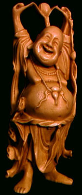
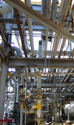
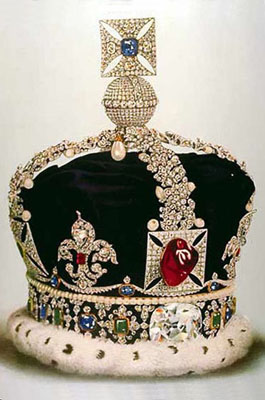
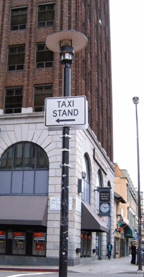
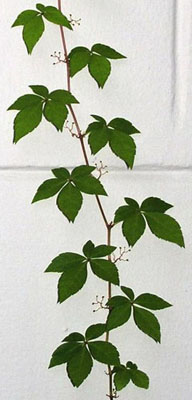
A wood statue	A whole oil-refinery	A museum piece	Downtown Berkeley	A vine on a wall

(Static) photo-realistic rendering is mostly a solved problem;
making suitable CG-models is not !

Distingquish between generated and aquired models,
and between pure 3D models, image/texture-enhanced (coarse) 3D models, and image-based models.

Model Generation versus Reality Acquisition

Remember the modeling paradigms: CSG, B-rep, voxels, instantiations ...
Those representations could be created by hand or in some procedural manner:

CS 184: Instantiations Sweeps Subdivision surfaces

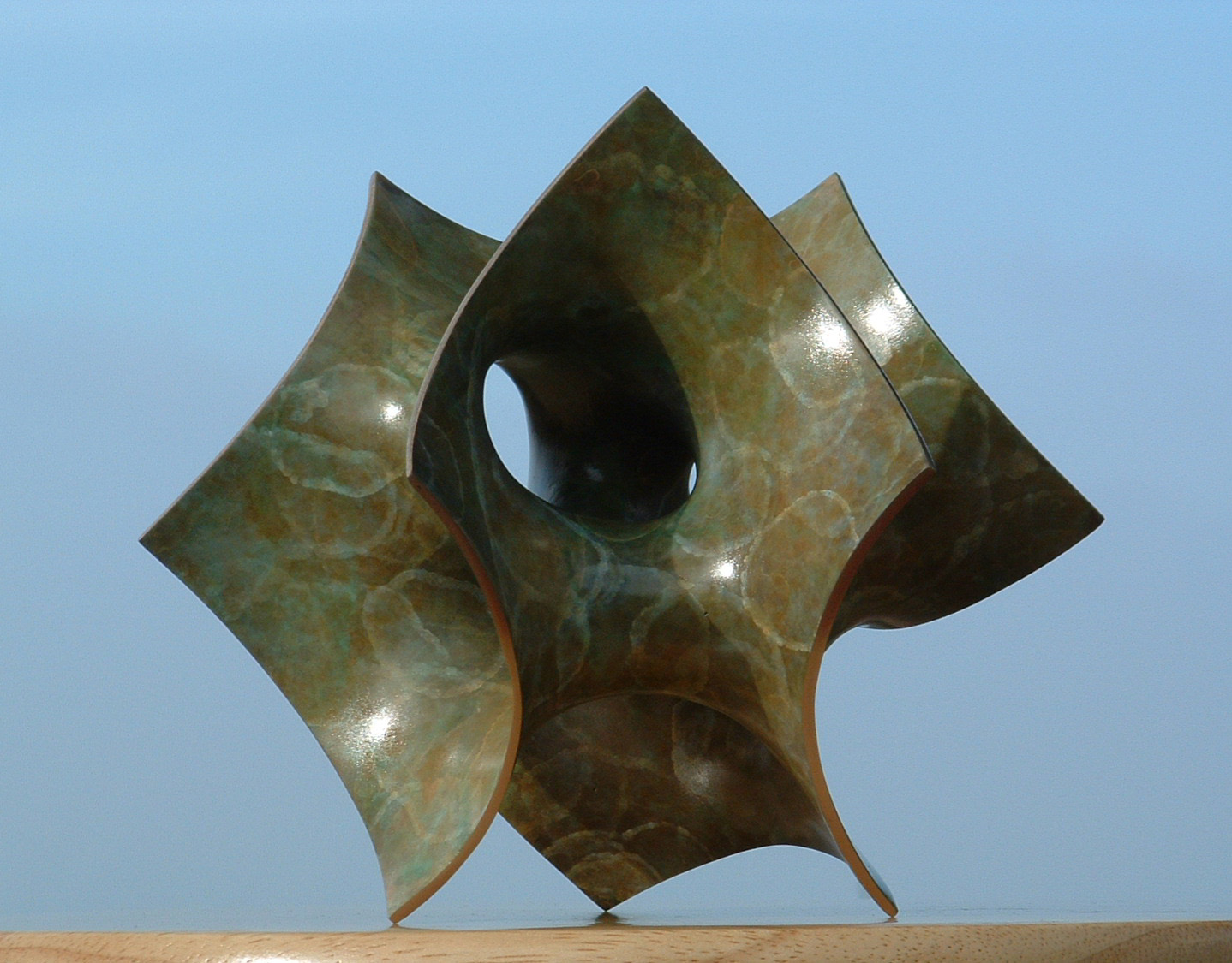
CS 284: Minimal surfaces Optimized MVS Sculpture generator

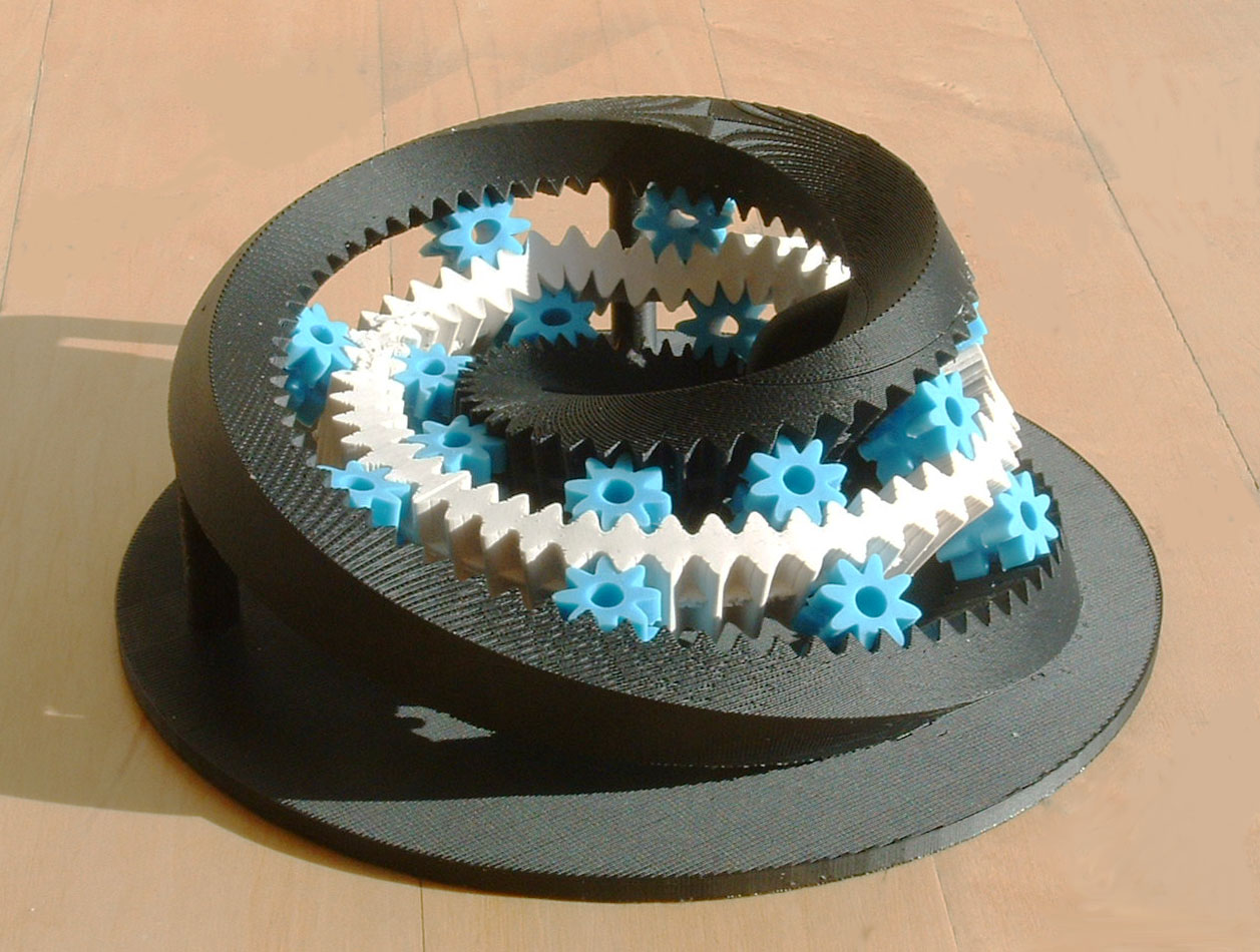
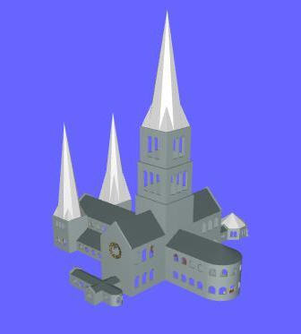
CS 285: Gear generator Church builder L-systems Phyllotaxis

However, some other objects that we would like to present on a computer screen (on a web page, or in a movie) are very difficult to model with just polygons, e.g., complex museum pieces made from many difficult-to-render materials (including velvet, precious jewels, surfaces with structural interference colors ...). One might then try to make models from photographs or by using a 3D scanner, or both. The final goal is to create a CG-model of some sort that can then be viewed from arbitrary viewpoints and with different illuminations.

In all image-based/enhanced models, sampling issues are of crucial importance (last lecture!)

Image-Based Rendering

Here, no 3D model of a scene to be rendered exists, only a set of images taken from several different locations.
For two "stereo pictures" taken from two camera locations that are not too far apart,
correspondence is established between key points in the two renderings (either manually, or with computer vision techniques).

By analyzing the differences of their relative positions in the two images, one can extract 3D depth information.
Thus groups of pixels in both images can be annotated with a distance from the camera that took them.
This basic approach can be extended to many different pictures taken from many different camera locations.
The depth annotation establishes an implicit 3D database of the geometry of the model object or scene.
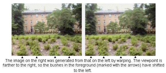
Pixels at different depths then get shifted by different amounts.

To produce a new image from a new camera location, one selects images taken from nearby locations
and suitably shifts or "shears" the pixel positions according to their depth and the difference in camera locations.
The information from the various nearby images is then combined in a weighted manner,
where closer camera positions, or the cameras that see the surface of interest under a steeper angle, are given more weight.
With additional clever processing, information missing in one image (e.g., because it is hidden behind a telephone pole)
can be obtained from another image taken from a different angle,
or can even be procedurally generated by extending nearby texture patterns.

Example 1: Stereo from a single source: A depth-annotated image of a 3D object, rendered from two different camera positions.
Example 2: Interpolating an image from neighboring positions:

To Learn More: UNC Image-Based Rendering
Future Graduate Courses: CS 283, CS 294-?

Image Warping (re-projection) and Stitching

Images taken from the same location, but at different camera angles need to be warped before they can be stitched together:
The original two photos at different angles. The final merged image.

To Learn More: P. Heckbert's 1989 MS Thesis: Fundamentals of Texture Mapping and Image Warping.

Light Field Rendering

How many images are enough to give "complete" information about all visual aspects of an object or scene ?
Let's consider the (impler) case of a relatively small, compact "museum piece" that we would like to present
to the viewers in a "3D manner" so that they can see it from (a range of) different angles.
Let's consider a few eye positions to view the crown. How many camera positions need to be evaluated ?

Light field methods use another way to store the information acquired from a visual capture of an object.
If one knew the complete 4D plenoptic function (all the photons traveling in all directions at all points in space surrounding an object),
i.e., the visual information that is emitted from the object in all directions into the space surrounding it,
then one could reconstruct perfectly any arbitrary view of this object from any view point in this space.

As an approximation, one captures many renderings from many locations (often lying on a regular array of positions and directions),
ideally, all around the given model object, but sometimes just from one dominant side.
This information is then captured in a 4D sampled function (2D array of locations, with 2D sub arrays of directions).
One practical solution is to organize and index this information (about all possible light rays in all possible directions)
by defining the rays by their intercept coordinates (s,t) and (u,v) of two points lying on two parallel planes.
The technique is applicable to both synthetic and real worlds, i.e. objects they may be rendered or scanned.
Creating a light field from a set of images corresponds to inserting 2D slices into the 4D light field representation.
Once a light field has been created, new views may be constructed by extracting 2D slices in appropriate directions,
i.e., by collecting the proper rays that form the desired image, or a few close-by images that can be interpolated.

"Light Field Rendering":
Example: Image shows (at left) how a 4D light field can be parameterized by the intersection of lines with two planes in space.
At center is a portion of the array of images that constitute the entire light field. A single image is extracted and shown at right.
Source: http://graphics.stanford.edu/projects/lightfield/

To Learn More: Light Field Rendering by Marc Levoy and Pat Hanrahan
Future Graduate Courses: CS 283, CS 294-?

3D Scanning

If we are primarily concerned with the 3D geometry of the object or scene to be modeled, then we may use a 3D scanner
Such a device takes an "image" by sampling the scene like a ray-casting machine,
but which also returns for each pixel the distance from the scanner.
This collection of 3D points is then converted into a geometrical model, by connecting neighboring sample dots
(or a subset thereof) into 3D meshes.
Color information can be associated with all vertices, or overlaid as a texture taken from a visual image of the scene.
This all requires quite a bit of work, but it results in a traditional B-rep model that can be rendered with classical techniques.
Challenges: To combine the point clouds taken from many different directions into one properly registered data set,
and to reduce the meshes to just the "right number" of vertices, and to clean up the "holes" in the resulting B-rep.
Example: Happy Buddha.

If we want to acquire internal, inaccessible geometry, e.g., of a brain, or a fetus, or of the bone structure of a living creature, we may use a computer tomography technique (MRI or ultra sound) that returns a 3D raster of data points with some variable, acquired value such as density, or water content. To make this data visible in a reasonable manner, we then need some different rendering techniques from what we have discussed in this course.
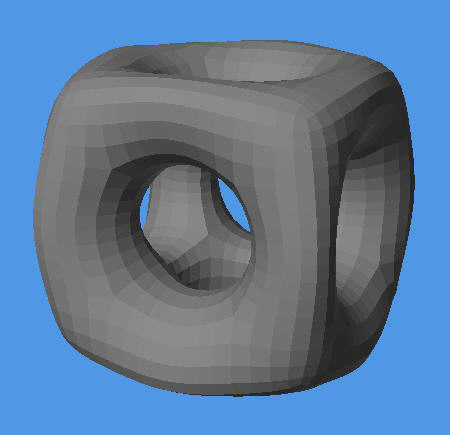
One apprach is to define some threshold on the measured variable (e.g. denisty), and declare all 3D raster points with values above this threshold as "inside" and all others as "outside." We can then generate a surface between the inside and the outside points (interpolate surface between sample points), for instance with an algorithm called Marching Cubes.
This reconstructed surface can then be rendered with any of the rendering techniques that we have discussed.

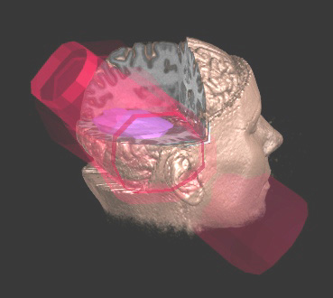
Volume Rendering

Alternatively, we might want to see details throughout the whole volume.
Then we need to render all the 3D raster data like some partly transparent fog with variable opacity,
or like nested bodies of "jello" of different colors and transparencies, which can then be rendered with raytracing methods.

The Volume Rendering technique can directly display sampled 3D data without first fitting geometric primitives to the samples.
In one approach, surface shading calculations are performed at every voxel using local gradient vectors to determine surface normals.
In a separate step, surface classification operators are applied to obtain a partial opacity for every voxel,
so that contour surfaces of constant densities or region boundary surfaces can be extracted.
The resulting colors and opacities are composited from back to front along the viewing rays to form an image.
(Remember lecture on transparency )
The goal is to develop algorithms for displaying this sort of data which are efficient and accurate, so that one can hope to obtain
photorealistic real-time volume renderings of large scientific, engineering, or medical datasets on affordable non-custom hardware.

Example: Scull and Brain
Source: http://graphics.stanford.edu/projects/volume/

Rapid Prototyping

Finally, you should not see computer graphics to be limited to just producing 2D output in terms of pretty pictures and animations.
Via rapid prototyping machines, computer graphics models can be turned into real, tangible 3D artifacts.
Most of these machines work on the principle of layered manufacturing, building up a 3D structure layer by layer,
by depositing some tiny particles of material or by selectively fusing or hardening some material already present.

To Learn More: Graduate Course: CS 285

My Own Use of Computer Graphics

PDF of the slides of a longer guest lecture given in the past

Where to go from here ... ?

Undergraduate Courses:

CS 160 User Interfaces
CS 194 The Art of Animation (Prof. Barsky)
CS 194 Advanced Digital Animation (Prof. Barsky+Dr. Garcia)

Graduate Courses:

CS 260 User Interfaces to Computer Systems
CS 274 Computational Geometry
CS 280 Computer Vision
"CS 283" or CS 294-? a new core graduate course in graphics (Fall 2009: Profs. O'Brien + Ramamoorthi)
CS 284 Computer-Aided Geometric Design (Fall 2009: Prof. Séquin)

Specialty Graduate Courses (taught about every 2-3 years):

CS 285 Solid free-form modeling and rapid prototyping (Prof. Séquin)
CS 294-? Mesh generation and geometry processing (Prof. Shewchuk)
CS 294-? Physically-based animation (Prof. O'Brien)
CS 294-? Visualization (Prof. Agrawala)
CS 294-? Design realization and pototyping (Prof. Canny)
CS 294-? Design of health technology (Prof. Canny)
CS 294-? an advanced rendering course (Prof. Ramamoorthi)

Final Exam: Friday, May 15, from 5pm till 8pm, in 360 SODA HALL

Rules: This is what you will see on the front page:

INSTRUCTIONS ( Read carefully ! )

DO NOT OPEN UNTIL TOLD TO DO SO !

TIME LIMIT: 170 minutes. Maximum number of points: ____.

CLEAN DESKS: No books; no calculators or other electronic devices; only writing implements
and TWO double-sided sheet of size 8.5 by 11 inches of your own personal notes.

NO QUESTIONS ! ( They are typically unnecessary and disturb the other students.)
If any question on the exam appears unclear to you, write down what the difficulty is
and what assumptions you made to try to solve the problem the way you understood it.

DO ALL WORK TO BE GRADED ON THESE SHEETS OR THEIR BACKFACES.

NO PEEKING; NO COLLABORATION OF ANY KIND!

I HAVE UNDERSTOOD THESE RULES:

Your Signature:___________________________________

Advice on Exam Preparation

Think through the topics covered in this course.

Prepare one additional sheet of notes to be used during the exam.

The TA's have offered to hold review discussion sessions at the regular times on Monday and Tuesday, May 11 and 12:

Project Demonstrations:
Tuesday and Wednesday, May 19/20, 2009 in 330 Soda Hall

Each group MUST demonstrate their final project.
Sign up for a 12-minute time slot:
    -- Tue 5/19: 2pm-5pm
    -- Wed 5/20: 10am-12noon
    -- Wed 5/20: 2pm-4pm
       A sign-up list will be posted on the instructional web page:       http://inst.eecs.berkeley.edu/~cs184/sp09/signup/
Demos will take place in 330 Soda. Make sure your demo is ready to run at the start of your assigned demo slot;
Bring a hard copy of the project score sheet filled in with the name(s), login(s) and demo time slot for your team;
also fill in your best estimate of what you think you have achieved.

Final Project Submission:

Submit your project as you did your assignments (for the record) -- within one hour after your demo time.

Create a project webpage in your personal directory of your cs184 account
that includes a descriptive paragraph and screenshot. (Also include this information in your submission.)