Contents

Line (Trapezoid)

disp('######################################');
disp('#### Design a circular trajectory ####');
disp('####                              ####');
disp('######################################');
disp(' ');
kx = linspace(-5,5, 256)';
ky = linspace(-5,5, 256)';
kz = 0*ky;
C = [kx ky kz];

[C_riv, time_riv, g_riv, s_riv, k_riv] = minTimeGradient(C,0, 0, 0, 4, 15, 4e-3);          % Rotationally invariant solution
[C_rv, time_rv, g_rv, s_rv, k_rv] = minTimeGradient(C,1, 0, 0, 4, 15, 4e-3);     % Rotationally variant solution

L = max(length(s_riv), length(s_rv));

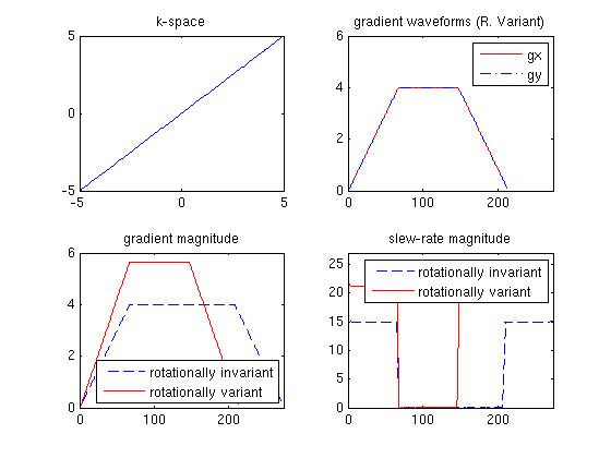
figure, subplot(2,2,1), plot(C_rv(:,1), C_rv(:,2)); title('k-space'); axis([-5 5 -5 5]);
subplot(2,2,2), plot(g_rv(:,1), 'r'); axis([0,L,-4.5,4.5]); title('gradient waveforms (R. Variant)'); axis([0 L 0 6]);
hold on, subplot(2,2,2), plot(g_rv(:,2), '-.');
legend('gx', 'gy', 'Location', 'NorthEast');
subplot(2,2,3), plot((g_riv(:,1).^2 + g_riv(:,2).^2).^0.5, '--'),
hold on, subplot(2,2,3), plot((g_rv(:,1).^2 + g_rv(:,2).^2).^0.5, 'r');   axis([0 L 0 6]);
legend('rotationally invariant', 'rotationally variant', 'Location', 'SouthEast'); title('gradient magnitude')
subplot(2,2,4), plot((s_riv(:,1).^2 + s_riv(:,2).^2).^0.5, '--'); title('slew-rate magnitude'); axis([0 L 0 27]);
hold on, subplot(2,2,4), plot((s_rv(:,1).^2 + s_rv(:,2).^2).^0.5, 'r');
legend('rotationally invariant', 'rotationally variant', 'Location', 'NorthEast');

######################################
#### Design a circular trajectory ####
####                              ####
######################################
 
Computing the rotationally invariant solution
Compute geometry dependent constraints 
Solving ODE Forward
Solving ODE Backwards
Final interpolation
Done
Computing the rotationally variant solution
Compute geometry dependent constraints 
Solving ODE Forward
Solving ODE Backwards
Done

Circle

disp('######################################');
disp('#### Design a circular trajectory ####');
disp('####                              ####');
disp('######################################');
disp(' ');

C = exp(i*2*pi*linspace(0,1,512)')*10;
C = [real(C) imag(C) 0*C];
[C_riv, time_riv, g_riv, s_riv, k_riv] = minTimeGradient(C,0);          % Rotationally invariant solution
[C_rv, time_rv, g_rv, s_rv, k_rv] = minTimeGradient(C,1, 0);  % Rotationally variant solution

L = max(length(s_riv), length(s_rv));

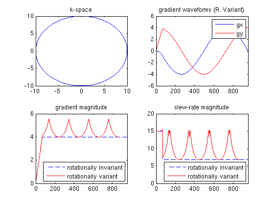
figure, subplot(2,2,1), plot(C_rv(:,1), C_rv(:,2)); title('k-space'); axis([-10 10 -10 10]);
subplot(2,2,2), plot(g_riv(:,1)); axis([0,L,-4.5,4.5]); title('gradient waveforms (R. Variant)'); axis([0 L -6 6]);
hold on, subplot(2,2,2), plot(g_riv(:,2), 'r');
legend('gx', 'gy', 'Location', 'NorthEast');
subplot(2,2,3), plot((g_riv(:,1).^2 + g_riv(:,2).^2).^0.5, '--'),
hold on, subplot(2,2,3), plot((g_rv(:,1).^2 + g_rv(:,2).^2).^0.5, 'r'); axis([0 L 0 6]);
legend('rotationally invariant', 'rotationally variant', 'Location', 'SouthEast'); title('gradient magnitude')
subplot(2,2,4), plot((s_riv(:,1).^2 + s_riv(:,2).^2).^0.5, '--'); title('slew-rate magnitude'); axis([0 L 0 20]);
hold on, subplot(2,2,4), plot((s_rv(:,1).^2 + s_rv(:,2).^2).^0.5, 'r');
legend('rotationally invariant', 'rotationally variant', 'Location', 'SouthEast');

######################################
#### Design a circular trajectory ####
####                              ####
######################################
 
Computing the rotationally invariant solution
Compute geometry dependent constraints 
Solving ODE Forward
Solving ODE Backwards
Final interpolation
Done
Computing the rotationally variant solution
Compute geometry dependent constraints 
Solving ODE Forward
Solving ODE Backwards
Done

Spiral

disp('######################################');
disp('#### Design a dual density spiral ####');
disp('####                              ####');
disp('######################################');
disp(' ');

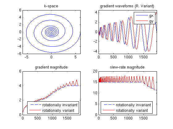
[k_rv,g_rv,s_rv,time_rv,Ck_rv] = vdSpiralDesign(1, 16, 0.83,[55,55,10,10],[0,0.2,0.3,1],4,15,4e-3,'cubic');
[k_riv,g_riv,s_riv,time_riv,Ck_riv] = vdSpiralDesign(0, 16, 0.83,[55,55,10,10],[0,0.2,0.3,1],4,15,4e-3,'cubic');

L = max(length(s_riv), length(s_rv));
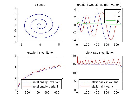
figure, subplot(2,2,1), plot(k_rv(:,1), k_rv(:,2)); title('k-space'); axis([-6 6 -6 6]);
subplot(2,2,2), plot(g_riv(:,1)); axis([0,L,-4.5,4.5]); title('gradient waveforms (R. Variant)')
hold on, subplot(2,2,2), plot(g_riv(:,2), 'r');
legend('gx', 'gy', 'Location', 'NorthEast');
subplot(2,2,3), plot((g_riv(:,1).^2 + g_riv(:,2).^2).^0.5, '--'),
hold on, subplot(2,2,3), plot((g_rv(:,1).^2 + g_rv(:,2).^2).^0.5, 'r');  axis([0 L 0 6]);
legend('rotationally invariant', 'rotationally variant', 'Location', 'SouthEast'); title('gradient magnitude')
subplot(2,2,4), plot((s_riv(:,1).^2 + s_riv(:,2).^2).^0.5, '--'); title('slew-rate magnitude');  axis([0 L 0 20]);
hold on, subplot(2,2,4), plot((s_rv(:,1).^2 + s_rv(:,2).^2).^0.5, 'r');
legend('rotationally invariant', 'rotationally variant', 'Location', 'SouthWest');

######################################
#### Design a dual density spiral ####
####                              ####
######################################
 
Computing the rotationally variant solution
Compute geometry dependent constraints 
Solving ODE Forward
Solving ODE Backwards
Done
Computing the rotationally invariant solution
Compute geometry dependent constraints 
Solving ODE Forward
Solving ODE Backwards
Final interpolation
Done

Rosette

disp('############################################');
disp('#### Design a rosette trajectory        ####');
disp('####                                    ####');
disp('############################################');
disp(' ');

Gmx = 4;
Smx = 15;
T = 17/Gmx;
Kmx = 6;
w1 = 0.147*2*pi*Gmx;
w2 = 0.087/1.02*2*pi*Gmx;
t = 0e-3:4e-3:T;
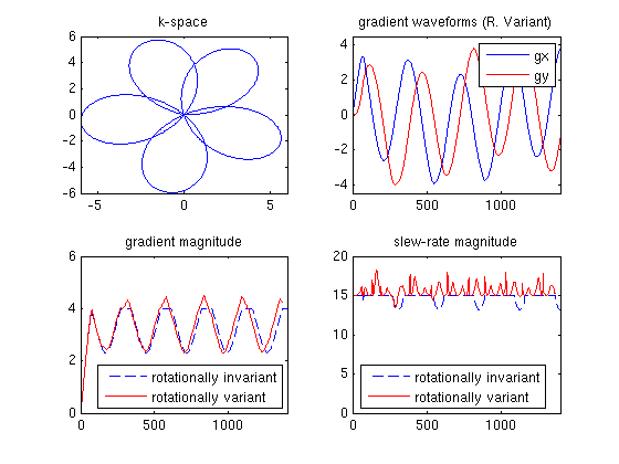
C = Kmx*sin(w1*t').*exp(i*w2*t');
C = [real(C) imag(C) 0*C];

[C_riv, time_riv, g_riv, s_riv, k_riv] = minTimeGradient(C,0);          % Rotationally invariant solution
[C_rv, time_rv, g_rv, s_rv, k_rv]= minTimeGradient(C,1, 0);  % Rotationally variant solution
L = max(length(s_riv), length(s_rv));

figure, subplot(2,2,1), plot(C_rv(:,1), C_rv(:,2)); title('k-space'); axis([-6 6 -6 6]);
subplot(2,2,2), plot(g_riv(:,1)); axis([0,L,-4.5,4.5]); title('gradient waveforms (R. Variant)')
hold on, subplot(2,2,2), plot(g_riv(:,2), 'r');
legend('gx', 'gy', 'Location', 'NorthEast');
subplot(2,2,3), plot((g_riv(:,1).^2 + g_riv(:,2).^2).^0.5, '--'),
hold on, subplot(2,2,3), plot((g_rv(:,1).^2 + g_rv(:,2).^2).^0.5, 'r');  axis([0 L 0 6]);
legend('rotationally invariant', 'rotationally variant', 'Location', 'SouthEast'); title('gradient magnitude')
subplot(2,2,4), plot((s_riv(:,1).^2 + s_riv(:,2).^2).^0.5, '--'); title('slew-rate magnitude');  axis([0 L 0 20]);
hold on, subplot(2,2,4), plot((s_rv(:,1).^2 + s_rv(:,2).^2).^0.5, 'r');
legend('rotationally invariant', 'rotationally variant', 'Location', 'SouthWest');

############################################
#### Design a rosette trajectory        ####
####                                    ####
############################################
 
Computing the rotationally invariant solution
Compute geometry dependent constraints 
Solving ODE Forward
Solving ODE Backwards
Final interpolation
Done
Computing the rotationally variant solution
Compute geometry dependent constraints 
Solving ODE Forward
Solving ODE Backwards
Done

Cone

disp('############################################');
disp('####   Design a cone trajectory         ####');
disp('####                                    ####');
disp('############################################');
disp(' ');

r = linspace(0,5, 512)';
th = linspace(0,2*pi, 512)';
C = r.*exp(3*1i*th);
C = [real(C) imag(C) r];
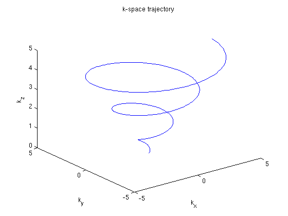
figure, plot3(C(:,1), C(:,2), C(:,3))
title('k-space trajectory')
xlabel('k_x'); ylabel('k_y'); zlabel('k_z');

[C_rv, time_rv, g_rv, s_rv, k_rv] = minTimeGradient(C,0);          % Rotationally variant solution
[C_riv, time_riv, g_riv, s_riv, k_riv] = minTimeGradient(C,1, 0);  % Rotationally invariant solution
L = max(length(s_riv), length(s_rv));

figure, subplot(2,2,1), plot3(C_rv(:,1), C_rv(:,2), C_rv(:,3)); title('k-space'); axis([-6 6 -6 6]);
subplot(2,2,2), plot(g_riv(:,1)); axis([0,L,-4.5,4.5]); title('gradient waveforms (R. Invariant)')
hold on, subplot(2,2,2), plot(g_riv(:,2), 'r');
hold on, subplot(2,2,2), plot(g_riv(:,3), 'g');
legend('gx', 'gy', 'gz', 'Location', 'NorthEast');
subplot(2,2,3), plot((g_rv(:,1).^2 + g_rv(:,2).^2).^0.5, '--'),
hold on, subplot(2,2,3), plot((g_riv(:,1).^2 + g_riv(:,2).^2).^0.5, 'r');  axis([0 L 0 6]);
legend('rotationally invariant', 'rotationally variant', 'Location', 'SouthEast'); title('gradient magnitude')
subplot(2,2,4), plot((s_rv(:,1).^2 + s_rv(:,2).^2+ s_rv(:,3).^2).^0.5, '--'); title('slew-rate magnitude');  axis([0 L 0 20]);
hold on, subplot(2,2,4), plot((s_riv(:,1).^2 + s_riv(:,2).^2+ s_riv(:,3).^2).^0.5, 'r');
legend('rotationally invariant', 'rotationally variant', 'Location', 'SouthWest');

############################################
####   Design a cone trajectory         ####
####                                    ####
############################################
 
Computing the rotationally invariant solution
Compute geometry dependent constraints 
Solving ODE Forward
Solving ODE Backwards
Final interpolation
Done
Computing the rotationally variant solution
Compute geometry dependent constraints 
Solving ODE Forward
Solving ODE Backwards
Done

Published with MATLAB® 7.8