For example, in an earlier lecture on solving the discrete Poisson equation, we presented a table of complexities of solving this equation on an n-by-n grid (a linear system A*x=b with N=n2 unknowns). Treating the matrix A as dense leads to an algorithm taking O(N3) flops.
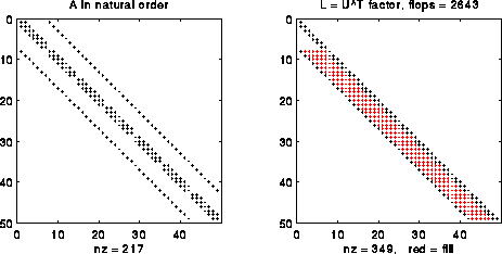
The simplest way to exploit sparsity in A is to treat is as a band matrix, with nonzeros only in a diagonal band 2n+1 diagonals wide (see the picture below). It turns out that we can do Gaussian elimination without pivoting on A (reordering the rows of A for numerical stability reasons); we discuss why below. In this case, we can show that it is possible to implement Gaussian elimination so as to
For example, the following figure shows the matrix A for a 7-b-7 grid (a 49-by-49 matrix) and its factors A = L*U. In this case, we can take L=UT, a variation of Gaussian elimination called Cholesky (see below for details). The nonzero entries of L that are not also nonzero entries of A are called fill-in, and are colored red in the figure. The number of nonzero entries is given as "nz=..." in the captions. The number of floating point operations (done only on nonzero operands) is also given in the title as "flops= ...". As can be seen, the number of nonzeros is 349/(.5*492) = .3 of what a dense triangular matrix would require, and costs about 2643/(493/3) = .067 times as many flops.

Given L and U, we would then go ahead and solve A*x = L*U*x = b by solving the two triangular systems L*y = b for y and U*x = y for x.
Alternatively, we could consider solving the equivalent permuted linear system PAPTPx = Pb, or A1*x1=b1. Here P is a permutation matrix (so PTP = I), and b1 = P*b, i.e. b1 has the same entries as b but in permuted order. Similarly x1=P*x, i.e. x1 is x permuted the same way as b1. Finally, A1=P*A*PT, or A with its rows and columns permuted the same way as x1 and b1. If A is symmetric, so is A1. In the following figure, we consider a special permutation P called nested dissection ordering, which is computed using the graph partitioning algorithms we discussed in earlier lectures, and which we will explain in more detail below. Note that L has fewer nonzeros (288 nonzeros versus 349) and requires fewer flops to compute (1926 versus 2643).
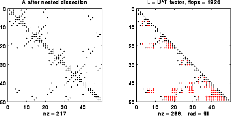
The savings from permuting grow as n grows. For example, with n=63 (N = n2 = 3969), the nonzero count is 250109 versus 85416, and the flop count is about 16 million versus 3.6 million, for the "natural" order versus "nested dissection" order, respectively. More generally, one can show that with nested dissection the storage grows like O(N log N) versus O(N2) for natural order, and the flop count grows like O(N3/2) versus O(N2). Indeed, it is a fact that "nested dissection" order is asymptotially optimal, in the sense that the functions O(N log N) and O(N3/2) can be made no smaller by any other choice of permutation P.
Later, we will also see that nested dissection also leads to significantly more parallelism than the natural order.
      A = [ eps  1  ]    where eps is 0 or very small.
          [  1  eps ]
There is an important class of matrices, which includes the discrete Poisson equation, where this factorization simplifies considerably. We define a matrix A to be symmetric positive definite (spd) if it is symmetric A = AT and positive definite (all its eigenvalues are positive). Equivalent definitions of positive definiteness are that the determinants of all leading principal submatrices are positive (det(A(1:i,1:i))>0 for i=1,...,n), and that A has a square root L, such that L is lower triangular and A = L*LT.
This last equivalent definition implies that we can do Gaussian elimination A = L*U without pivoting, and furthermore take UT=L. The factorization A = L*LT is called the Cholesky factorization, and L is called the Cholesky factor of L.
An operation count reveals that Cholesky on a dense spd matrix requires half the flops (n3/3 versus 2*n3/3) as standard Gaussian elimination, and also requires only half the space, since only the lower triangle of A and L must be stored. Symmetric positive definite matrices are extremely common in applications (for example, as mass and stiffness matrices in structural mechanics).
If A is spd, then so is P*A*PT for any permutation matrix P. This is true because P*A*PT is symmetric if A is, and also has the same (positive) eigenvalues as A. Thus, Cholesky works on A if and only if it works on P*A*PT for any P. We can equivalently say that Cholesky works equally well with any diagonal pivoting scheme, since P*A*PT, which is A with the same permutation applied to its rows and its columns, has the same diagonal as A but in a permuted order determined by P. As mentioned above, the correct choice of P can greatly impact
It turns out that sparse Cholesky is significantly simpler to implement than sparse Gaussian elimination with pivoting, because the choice of permutation matrix P does not depend on intermediate values computed during the factorizationi process, and so can be determined ahead of time to optimize the three quantities listed above. For this reason, we will initially concentrate on sparse Cholesky, and return to sparse Gaussian elimination with pivoting in a future lecture.
For sparse Cholesky, we can divide the implemenation into 4 phases:
( i, j, aij, next_i, last_i, next_j, last_j )where next_i points to the next nonzero entry in column j below i, last_i points to the previous nonzero entry in column j above i, and next_j and last_j similarly point to the neighboring nonzero entries in the same row.
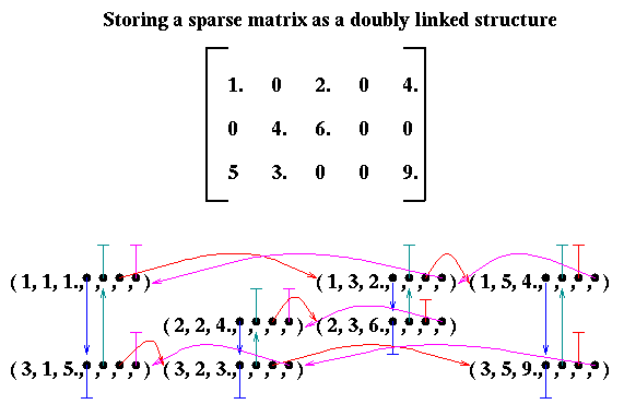
Indeed, by thinking of A as a block matrix
       [ A11  ...  A1n ]
   A = [ ...  ...  ... ]
       [ An1  ...  Ann ]
where the Aij are submatrices which could themselves be sparse,
we see that we could represent A hierarchically, with one scheme
to represent the subset of nonzero submatrices Aij present in A,
and other schemes for each Aij.
The otherwise very flexible linked list scheme has two drawbacks. First, it requires as much as 7 times as much storage as needed just for the nonzero entries themselves. Second, there is no memory locality, i.e. operating on a single row of m entries requires 2m memory accesses (to get the data and the next_i pointers) which may or may not be in nearby memory locations; recall that high performance in the presence of memory hierarchies requires that data to be accessed together be stored together.
Since algorithmic efficiency depends on storage scheme, most research has focused on choosing a scheme compatible with high performance. Matrices stored in different ways must first be converted to the scheme required by the algorithm. One of the basic storage schemes we will use is column compressed storage. This scheme stores the nonzero entries by column in one contiguous array called values. In addition, there is an equally long array row_ind of the row indices of each value (in otherwords, values(i) lies in row row_ind(i)). Finally, there is a (generally much shorter) array called col_ptr, indicating where in the values and row_ind arrays each column begins: column j starts at index col_ptr(j) (and ends at col_ptr(j+1)-1).
For example, the matrix above would be stored as follows:
           [ 1.  0   2.  0  4. ]
       A = [ 0   4.  6.  0  0  ]
           [ 5.  3.  0   0  9. ]

 values  = [ 1.  5.  4.  3.  2.  6.  4.  9. ]
 row_ind = [ 1   3   2   3   1   2   1   3  ]
 col_ptr = [ 1   3   5   7   7   9 ]
This storage scheme allows fast access to columns but not
rows of A, and requires about twice as much storage as
for the nonzero entries alone. Since it is not convenient
to access rows with this scheme, our algorithms using
this scheme will be column oriented.
Later we will discuss improvements on column compressed storage to enhance locality of memory accesses even more.
 ... for each column i,
 ... zero it out below the diagonal by
 ... adding multiples of row i to later rows
 for i = 1 to n-1
     ... each row j below row i
     for j = i+1 to n
         ... add a multiple of row i to row j
         for k = i to n
             A(j,k) = A(j,k) -
                     (A(j,i)/A(i,i)) * A(i,k)
Eliminating redundant work as in
Lecture 14 yields the algorithm
  for i = 1 to n-1
    for j = i+1 to n
        A(j,i) = A(j,i)/A(i,i)   ... store L on top of A
    for k = i+1 to n             ... we have also reversed the
        for j = i+1 to n         ... order of the j and k loops
            A(j,k) = A(j,k) - A(j,i) * A(i,k)
at the end of which A has been overwritten by L and U. To change this
into Cholesky, we proceed in two steps. First, we modify the algorithm
so that U=LT:
  for i = 1 to n-1
    A(i,i) = sqrt(A(i,i))  ... if error, A not positive definite
    for j = i+1 to n
        A(j,i) = A(j,i)/A(i,i)  ... store L on top of A
        A(i,j) = A(i,j)/A(i,i)  ... compute U in place too
    for k = i+1 to n
        for j = i+1 to n
            A(j,k) = A(j,k) - A(j,i) * A(i,k)
and then we use the fact that U=LT to eliminate all
references to the upper triangle of A:
  for i = 1 to n-1
    A(i,i) = sqrt(A(i,i))  ... if error, A not positive definite
    for j = i+1 to n
        A(j,i) = A(j,i)/A(i,i)  ... store col i of L on top of A
    for k = i+1 to n
        for j = k to n     ... update only on and below diagonal
            A(j,k) = A(j,k) - A(j,i) * A(k,i)  ... A(k,i)=A(i,k)
To simplify discussion, we abbreviate this algorithm as
  for i = 1 to n-1
    cdiv(i)   ... update column j
    for k = i+1 to n
        cmod(k,i)  ... update column k by column i
                   ... only necessary if A(k,i)=L(k,i) nonzero
Here cdiv(i) computes the final value of column i by performing
    A(i,i) = sqrt(A(i,i))  ... if error, A not positive definite
    for j = i+1 to n
        A(j,i) = A(j,i)/A(i,i)  ... store col i of L on top of A
and cmod(k,i) adds A(k,i) times column i to column k:
        for j = k to n     ... update only on and below diagonal
            A(j,k) = A(j,k) - A(j,i) * A(k,i)
It is important to note that cmod(k,i) does something useful
only if A(k,i) is nonzero. This is one of the ways we
exploit sparsity to avoid floating point operations
(the other way is to exploit sparsity in columns i and k
themselves).
To express this more formally, we define
Struct(L*i) = { k.gt.i such that Lki is nonzero }
In other words, Struct(L*i) is the list of row indices k
of the nonzero entries below the diagonal of column i of L.
It lists the columns to the right of i that depend on column i.
These are the only values of k for which we need to call cmod(k,i)
This lets us rewrite sparse Cholesky as
  for i = 1 to n-1
    cdiv(i)
    for k in Struct(L*i)
        cmod(k,i)
We call this version of Cholesky right-looking.
It is also sometimes called
fan-out,
submatrix,
or
data driven
Cholesky in the literature, because as soon as column
i is computed (by cdiv(i)), it is used to update all columns k to its
"right" that depend on it (i.e. column i is "fanned-out" to
update the "submatrix" to its right as soon as its "data" is available).
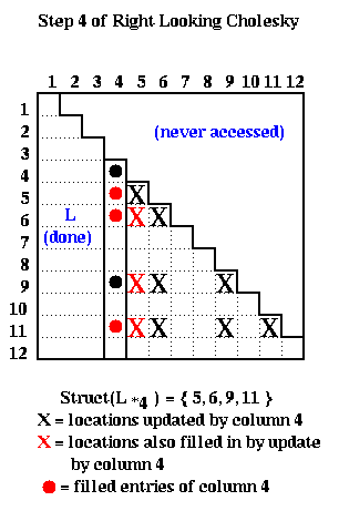
The following picture illustrates right-looking Choleksy on the 12-by-12 matrix shown below.
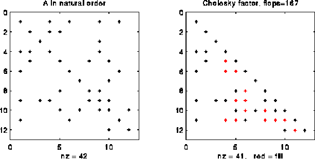
At step i=4 of right-looking Cholesky, columns 1 to 3 of L have been completed by the end of the previous step, cdiv(4) has been called to complete column 4 of L, and we are about to call cmod(k,4) for k in Struct(L*4) = { 7, 8, 11 }. The red and black Xs below mark the entries updated by the calls to cmod(7,4), cmod(8,4) and cmod(11,4).
Here is an alternative way to organize the algorithm. Instead of using column i to update all later columns that depend on it, so that any particular column is updated sporadically, as columns it depends on are completed, we perform all updates to column i at the same time, when all columns to its left are finished. To write this formally, we define
Struct(Lk*) = { i.lt.k such that Lki is nonzero }
Struct(Lk*) is a list of indices of
nonzeros in row k of L. It lists the columns to the left of k on which
column k depends. This lets us write the algorithm
  for k = 1 to n
    for i in Struct(Lk*)
        cmod(k,i)
    cdiv(k)
This version of Cholesky is called left-looking.
It is also sometimes called
fan-in
or
demand driven
Cholesky in the literature, because in order to compute column k,
we "fan-in" the columns to its "left" that it "demands" in order
to update itself.
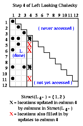
The following picture illustrates left-looking Choleksy at step k=4, on the same 12-by-12 matrix as above. At this point, columns 1 to 3 of L were completed by the end of the previous step, and we are about to call cmod(4,i) for i in Struct(L4*) = { 1, 2 }. The red and black Xs below mark the entries updated by the calls to cmod(4,1) and cmod(4,2). There is no fill-in in the first 3 columns of L; the first fill-in occurs in column 4 as indicated by the red Xs.
Right-looking and left-looking are not the only ways to organize the work done by Cholesky, but to discuss other options we need to explore the dependencies of columns on one another in more detail in the next section.
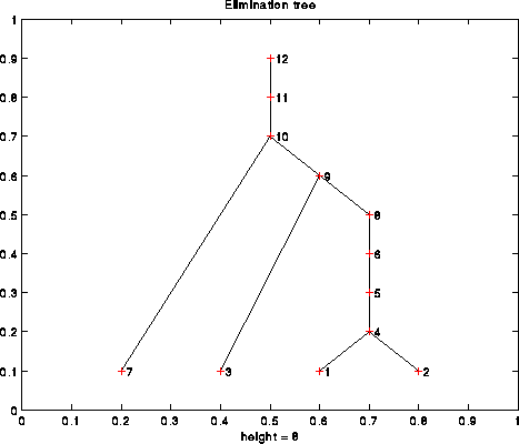
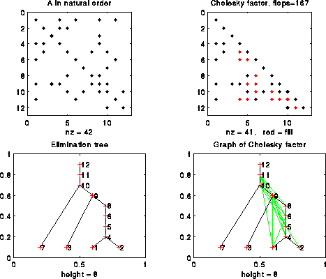
Let i be a column of A. We define parent(i) to be the index k of the first nonzero in Struct(L*i), i.e. the first nonzero below the diagonal in column i of L. Recalling how Cholesky works, this is the first column to the right of column i, that depends on column i. In particular, column i must be completely computed before column parent(i). This parent relationship defines the e-tree of A. For example, the following is the e-tree of the 12-by-12 matrix illustrated above:
Here is the basic fact about elimination trees, whose proof we omit.
Proposition. It is possible to compute the columns of the Cholesky factorization of A in any order consistent with computing the children c of column i in the e-tree before computing column i (a post-order traversal of the e-tree). In particular
This lets a write a "most general" version of sparse Cholesky, which includes all possible orderings (such as right-looking or left-looking) as special cases. The Task-Queue maintains a list of all tasks (cdiv(i) or cmod(k,i)) that are currently ready to execute:
  Task-Queue = {cdiv(i) for all leaves i of the e-tree}
  While Task-Queue not empty
    remove a task from the Task-Queue  ... any one will do
    if task = cdiv(i) then
       perform cdiv(i)
       for all k in Struct(L*i)
           add cmod(k,i) to Task-Queue
    else if task = cmod(k,i)
       perform cmod(k,i)
       if this was last cmod of column k,
            add cdiv(k) to Task-Queue
    endif
Depending on the order in which we remove tasks from the Task-Queue,
we could get a left-looking algorithm, a right-looking algorithm, or one of
many others.
In particular, since any task from the Task-Queue is ready to execute, a parallel algorithm could execute any subset of the tasks currently in the Task-Queue in parallel (note that if we try to execute cmod(k,i) and cmod(k,j) in parallel, both will try to update column k simultaneously, so some locking is needed to prevent a race condition). Thus, the above algorithm becomes a parallel algorithm if each processor executes it simulateously, with a common global Task-Queue from which processors remove and add tasks.
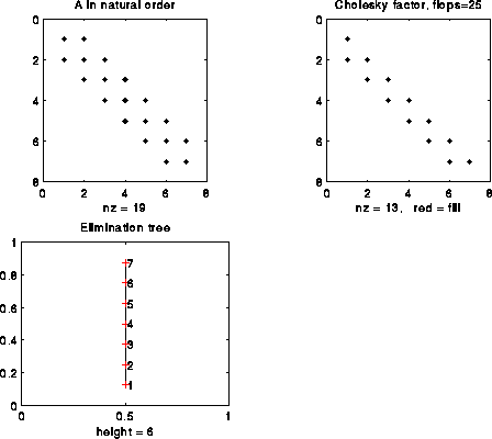
Let us illustrate this Proposition on some more examples. The figure below illustrates a 7-by-7 tridiagonal matrix in the natural order. In this simple example, where there is no fill-in, the e-tree is a simple chain, and tells us the simple and obvious fact that column i must be computed before column i+1.
Slightly more interesting is the following matrix, which is the same 7-by-7 tridiagonal matrix with its rows and columns permuted into the order [1 3 2 5 7 6 4]. We have also added a graph of the whole L factor in the bottom right, with green edges added to represent the entries of L that are not also tree edges (in other words, there is one edge per offdiagonal nonzero of L, or equivalently one edge per call to cmod):
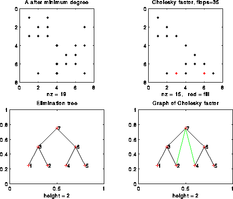
The reader may well ask what advantage there is in the second ordering, since there is more fill-in (2 versus 0) and more flops (35 versus 25). The advantage is parallelism, since the elimination tree is no longer a chain. In fact, since columns 1, 2, 4 and 5 have no children, they can be computed in parallel. Then, columns 3 and 6 can be computed in parallel, and finally column 7.
In other words, with enough processors (and memory bandwidth!) the time to perform sparse Cholesky in parallel depends essentially on the height of the elimination tree. (It is also possible to extract parallelism by having more than one processor participate in a single cdiv or cmod; we will discuss this later.)
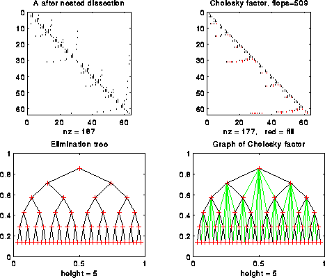
In general, for an n-by-n tridiagonal matrix, the natural order results in a chain of height n as an e-tree, taking n parallel steps to compute. In contrast, nested dissection yields an e-tree of height log2 n. (The reader may wish to compare this O(log2 n) solution of a tridiagonal system of equations with the one we presented based on parallel prefix.)
For example, the following figure shows n=127 with nested dissection ordering:
Here is our 12-by-12 example from earlier, including a graph of L:
We will see other examples below as well.
Furthermore, even achieving just one of these goals exactly is an NP-complete problem, meaning that the best known algorithms take a very long time to run, in fact asymptotically longer than dense Cholesky. So instead of exact solutions we will resort to heuristics.
It turns out that we have seen all but one of these heuristics before, in the context of graph partitioning. After explaining the one new heuristic minimum degree ordering we return to the others, Reverse Cuthill-McKee (which is closely related to breadth first search), and Nested Dissection (which can actually use any of the other graph partitioning algorithms discussed in Lectures 20, 21, or 23.