                        d^2 u(x,y)   d^2 u(x,y)
   2D-Laplacian(u)  =   ---------- + ----------  = f(x,y)
                          d x^2          d y^2
for (x,y) in a region Omega in the (x,y) plane,
say the unit square 0 < x,y < 1.
To make the solution well defined, we also need to specify boundary conditions,
i.e. the value of u(x,y) on the boundary of Omega. We will consider the
simple case
u(x,y) = 0 if (x,y) is on the boundary of OmegaThis equation describes the steady-state temperature of a uniform square plate with the boundaries held at temperature u=0, and f(x,y) equaling the external heat supplied at (x,y).
In 3 dimensions, the equation is quite similar,
                       d^2 u(x,y,z)   d^2 u(x,y,z)   d^2 u(x,y,z)
   3D-Laplacian(u)  =  ------------ + ------------ + ------------
                          d x^2           d y^2          d z^2

                    = f(x,y,z)
for (x,y,z) in a region Omega in (x,y,z) space.
Boundary conditions are also needed,
i.e. the value of u specified on the boundary of Omega.
For simplicity of presentation, we will discuss only the solution of Poisson's equation in 2D; the 3D case is analogous.
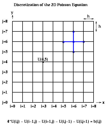
Recalling Lecture 13 again, we discretize this equation by using finite differences: We use an (n+1)-by-(n+1) grid on Omega = the unit square, where h=1/(n+1) is the grid spacing. We let U(i,j) be the approximate solution at x=i*h and y=j*h. This is shown below for n=7, including the system of linear equations it leads to:

The above linear equation relating U(i,j) and the value at its neighbors (indicated by the blue stencil) must hold for 1 <= i,j <= n, giving us N=n^2 equations in N unknowns. When (i,j) is adjacent to a boundary (i=1 or j=1 or i=n or j=n), one or more of the U(i+-1, j+-1) values is on the boundary and therefore 0. b(i,j) = -f(i*h,j*h)*h^2, the scaled value of the right-hand-side function f(x,y) at the corresponding grid point (i,j).
To write this as a linear system in the more standard form P*Uhat = bhat, where Uhat and bhat are column vectors, we need to choose a linear ordering of the unknowns U(i,j). For example, the natural row ordering shown below
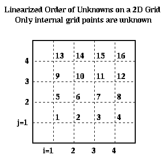
leads to the linear system P*Uhat = bhat:
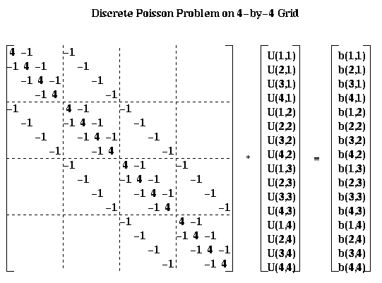
For the most part, we will describe our algorithms in term of the square array U(i,j) rather than the column vector Uhat. But for analysis it is convenient to be able to describe the algorithms using both formulations.
The first column in the table identifies the algorithm, except the last entry, which gives a simple Lower Bound on the running time for any algorithm. The Lower Bound is obtained as follows. For the serial time, the time required simply to print each of the N solution components is N. For the PRAM time, which assumes as many processors as we like and assumes communication is free, we note that the inverse inv(P) of the discrete Poisson matrix P is dense, so that each component of the solution Uhat = inv(P)*bhat is a nontrivial function of each of the N components of bhat. The time required to compute any nontrivial function of N values in parallel is log N.
The second column says whether the algorithm is of Type D=Direct, which means that after a finite number of steps it produces the exact answer (modulo roundoff error), or of Type I=Indirect, which means that one step of the algorithm decreases the error by a constant factor rho<1, where rho depends on the algorithm and N. This means that if one wants the final error to be epsilon times smaller than the initial error, one must take m steps where rho^m <= epsilon. To compute the complexities in the table, we choose m so that rho^m is about as small as the discretization error , i.e. the difference between the true solution x(i*h,j*h) and the exact discrete solution U(i,j). There is no point in making the error in the computed U(i,j) any smaller than this, since this could only decrease the more significant error measure, the difference between the true solution u(i*h,j*h) and the computed U(i,j), by a factor of 2.
The second and third columns give the running time for the algorithm on a serial machine and a PRAM, respectively. Recall that on a PRAM we can have as many processors as we need (shown in the last column), and communication is free. Thus, the PRAM time is a lower bound for any implementation on a real parallel machine. Finally, the fifth column indicated how much storage is needed. LU decomposition requires significantly more storage than the other methods, which require just a constant amount of storage per grid point.
   Algorithm   Type  Serial    PRAM          Storage  #Procs
                     Time      Time
   ---------   ----  ------    ---------     --------  ------
   Dense LU      D   N^3           N           N^2      N^2
   Band LU       D   N^2           N         N^(3/2)     N
   Inv(P)*bhat   D   N^2         log N         N^2      N^2
   Jacobi        I   N^2           N            N        N
   Sparse LU     D   N^(3/2)     N^(1/2)     N*log N     N
   CG            I   N^(3/2)   N^(1/2)*log N    N        N
   SOR           I   N^(3/2)   N^(1/2)          N        N
   FFT           D   N*log N     log N          N        N
   Multigrid     I   N           (log N)^2      N        N
   Lower Bound       N           log N          N

Key to abbreviations:
     Dense LU    : Gaussian elimination, treating P as dense
     Band LU     : Gaussian elimination, treating P as zero
                   outside a band of half-width n-1 near diagonal
     Sparse LU   : Gaussian elimination, exploiting entire
                   zero-structure of P
     Inv(P)*bhat : precompute and store inverse of P,
                   multiply it by right-hand-side bhat
     CG          : Conjugate Gradient method
     SOR         : Successive Overrelaxation
     FFT         : Fast Fourier Transform based method
We include methods like Dense LU (Gaussian Elimination) even though these are much slower than the fastest methods, because these slower methods solve much more general linear systems than the much faster but more specialized algorithms like Multigrid. This table illustrates that there is often an enormous payoff for using an algorithm specially tuned for the system at hand. Band LU is Gaussian Elimination specialized to take advantage of the fact that none of the zero entries of P more than n entries away from the diagonal ever "fill-in" during Gaussian Elimination, so we can avoid both storing them and doing arithmetic with them. Sparse LU exploits the fact that many other entries in the L and U factors of P are zero, and avoids both computing with or storing any zero entries; this requires interesting linked data structures we will discuss in later lectures. Inv(P)*bhat means precomputing and storing the exact N-by-N inverse of P (so we do not count the cost of this precomputation in the complexity), and then doing a matrix-vector multiplication. On a serial machine, this is no faster than any of the subsequent methods, and uses much more storage.
Jacobi, SOR (Successive OverRelaxation) and CG (Conjugate Gradients) can be thought of as performing most nearest neighbor operations on the grid (CG requires summing across the grid too). In other words, information at one grid point can only propagate to an adjacent grid point in 1 iteration. Since the solution U(i,j) at each grid point depends on the value of b(l,m) at every other grid point, it take n steps for information to propagate all the way across the grid. This would lead us not to expect a good solution in many fewer than n=sqrt(N) steps, which is what these methods require.
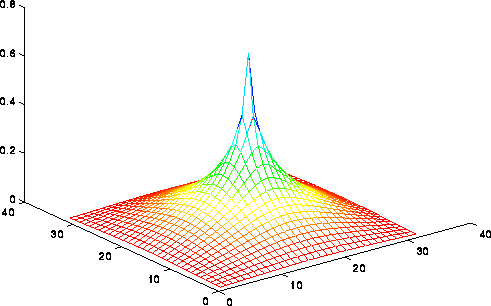
We can formalize this argument using the picture available here, or the less detailed picture below. Indeed, we can only show a lower bound of O(log n)=O(log N) steps for any "nearest neighbor" iterative method (rather than sqrt(n)). This picture shows the solution of the Poisson equation when b is zero expect for the value 1 in the center. The solution decays logarithmically from the center. If the solution could propagate only from grid point to grid point starting from 0 initial values, then after m < < n steps, one would still have a zero solution outside distance m from the center, even though the solution is large there; this means the error is large, and convergence is impossible. In fact, one can show that m=O(log n)=O(log N) steps are needed to multiply the error by a constant g<1, independent of n.
The FFT (Fast Fourier Transform) and Multigrid can be faster than nearest-neighbor methods because they move information across the grid in larger steps than merely between neighbors. It is interesting that Multigrid is asymptotically the fastest on a serial machine, attaining the lower bound of N steps. In contrast, FFT is fastest on a PRAM, attaining a lower bound of log N steps. One of our goals in the next two lectures is to do more detailed performance modeling of these methods, taking communication costs into account, to see which one we expect to be fastest in practice.
In addition to the methods in this table being in increasing order of speed for solving Poisson's equation, they are (roughly) in order of increasing specialization, in the sense that Dense LU can be used in principle to solve any linear system, whereas the FFT and Multigrid only work on equations quite similar to Poisson's equation. In practice, one wants the fastest method suitable for one's problem, and it often takes a great deal of specialized knowledge to make this decision. Fortunately, on-line help is available to help make this decision at the "templates" subdirectory of Netlib, especially the on-line book "Templates for the Solution of Linear Systems".
   U(i,j) =
      ( U(i-1,j) + U(i+1,j) + U(i,j-1) + U(i,j+1)
        + b(i,j) )/4
We let U(i,j,m) be our approximation for U(i,j) after the m-th iteration.
We can use any initial guess U(i,j,0); U(i,j,0)=0 will do. To get a
formula for U(i,j,m+1) in terms of the previous iteration U(i,j,m), we
simply use
   U(i,j,m+1) =
      ( U(i-1,j,m) + U(i+1,j,m) + U(i,j-1,m) + U(i,j+1,m)
        + b(i,j) )/4
In other words, U(i,j,m+1) is just a weighted average of its four
neighboring values and b(i,j).
We analyze the convergence rate of Jacobi as follows. We present only the final results; for details, see any good text on numerical linear algebra, such as "Lecture Notes on Numerical Linear Algebra", J. Demmel, Berkeley Lecture Notes in Mathematics, Mathematics Dept, UC Berkeley To state the result we define the error as the root-sum-of-squares of the error at each grid point:
error(m) = sqrt( sum_{ij} ( U(i,j,m) - U(i,j) )^2 )
It turns out that Jacobi decreases the error by a constant factor
rho_Jacobi(n) < 1, depending on dimension n, at each step:
   error(m) <= rho_Jacobi(n) * error(m-1)
            <= ( rho_Jacobi(n) )^m * error(0)
where
rho_Jacobi(n) = cos(pi/(n+1))When n is large, the interesting case, we can approximate rho_Jacobi(n) by
rho_Jacobi(n) ~ 1 - .5*(pi/(n+1))^2which gets closer to 1 as n grows. So to decrease the error by a factor of 2, say, requires taking m iterations where
      .5 > ( rho_Jacobi(n) )^m
         ~ ( 1 - .5*(pi/(n+1))^2 )^m
         ~ 1 - .5*(pi/(n+1))^2 * m     ... when n is large
or
m ~ ((n+1)/pi)^2In other words, convergence gets slower for large problems, with the number of steps proportional to N = n^2. This make the serial complexity
    Serial complexity of Jacobi
          = number_of_steps * cost_per_step
          = O(N) * O(N)
          = O(N^2)
This is easy to implement in parallel, because each grid cell value may
be updated independently. On a PRAM, this means the cost per step
is O(1), lowering the PRAM complexity to O(N).
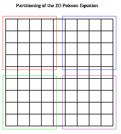
On a realistic parallel machine, one would simply assign grid point (i,j)
to processors in a block fashion as shown below, and have each processor
update the values of U(i,j,m+1) at the grid point it owns. This requires U
values on the boundary of the blocks to be communicated to neighboring
processors. When n >> p, so that each processor owns a large number n^2/p
of grid points, the amount of data communicated, n/p words with each neighbor,
will be relatively small.
To express the parallel running time in detail, we let
     p = number of processors
     f = time per flop
     alpha = startup for a message
     beta = time per word in a message
Then
  Time(Jacobi)
     = number_of_steps * cost_per_step
     = O(N) * ( (N/p)*f + alpha + (n/p)*beta )
     = O(N^2/p)*f + O(N)*alpha + O(N^(3/2) /p)*beta
where O(N/p) flops are needed to update local values,
alpha is the start up cost of messages to each neighbor, and
O(n/p) boundary values are communicated to neighbors.
Later we will compare this expression to similar expressions
for other methods.
The phenomenon of convergence slowing down, and needing to take more steps for large problems, is a common phenomenon for many methods and problems. It is not true for Multigrid, however, which takes a constant number of iterations to decrease the error by a constant factor, and so makes it very attractive.
The first improvement is motivated by examining the serial implementation, and noticing that while evaluating
  U(i,j,m+1)
      = ( U(i-1,j,m) + U(i+1,j,m) + U(i,j-1,m) + U(i,j+1,m)
          + b(i,j) )/4
new values for the solution at some of the grid points on the right hand side
are already available, and may be used. This leads to the algorithm
     U(i,j,m+1) = (U(i-1,j,latest) + U(i+1,j,latest) +
                   U(i,j-1,latest) + U(i,j+1,latest) + b(i,j) )/4
where "latest" is either m or m+1, depending on whether that particular
grid point has been updated already. This depends on the order in which
we loop through the (i,j) pairs. For example, if we use the same rowwise
ordering as in an earlier figure, we get the so-called Gauss-Seidel
algorithm:
   for i=1 to n
       for j=1 to n
           U(i,j,m+1) = (U(i-1,j,m+1) + U(i+1,j,m) +
                         U(i,j-1,m+1) + U(i,j+1,m) + b(i,j) )/4
       end for
   end for
This particular update order cannot be straightforwardly parallelized,
because there is a recurrence, with each U(i,j,m+1) depending on the
immediately previously updated value U(i-1,j,m+1).
So instead we loop through the grid points in the Red-Black order (named after the resemblance to a chess board) shown below.
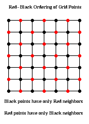
The idea is to update all the black points, followed by all the red points. The black grid points are connected only to red grid points, and so can all be updated simultaneously using the most recent red values. Then the red values can be updated using the most recent black values. This yields the following algorithm:
  for all black (i,j) grid points
      U(i,j,m+1) = (U(i-1,j,m) + U(i+1,j,m) +
                    U(i,j-1,m) + U(i,j+1,m) + b(i,j))/4
  end for
  for all red (i,j) grid points
      U(i,j,m+1) = (U(i-1,j,m+1) + U(i+1,j,m+1) +
                    U(i,j-1,m+1) + U(i,j+1,m+1) + b(i,j))/4
  end for
This can implemented in two parallel steps, one for updating the red points,
and one for the black.
By itself, this idea does not accelerate convergence. It turns out to converge twice as fast (rho_Gauss_Seidel(n) = rho_Jacobi(n)^2), but on a PRAM each parallel Gauss-Seidel step takes the same time as two parallel Jacobi steps, so there is no overall benefit.
The second improvement is called Successive Overrelaxation, and depends on the Red-Black ordering for its speedup. Let us rewrite the algorithm so far as
     U(i,j,m+1) = some_expression
                  ... an abbreviation for the
                  ... update scheme above
                = U(i,j,m) + (some_expression - U(i,j,m))
                = U(i,j,m) + correction(i,j,m)
The idea behind overrelaxation is that if correction(i,j,m) is a
good direction in which to move U(i,j,m) to make it a better solution,
one should move even farther in that direction, by a factor w>1:
U(i,j,m+1) = U(i,j,m) + w * correction(i,j,m)w is called the overrelaxation factor (w<1 would correspond to underrelaxation, which is not worth doing). The word successive refers to using the latest data to evaluate the correction.
Altogether, the SOR(w) algorithm is as follows:
  for all black (i,j) grid points
      U(i,j,m+1) = U(i,j,m) +
                   w * ( U(i-1,j,m) + U(i+1,j,m) +
                         U(i,j-1,m) + U(i,j+1,m) + b(i,j)
                         - 4*U(i,j,m) )/4
  end for

  for all red (i,j) grid points
      U(i,j,m+1) = U(i,j,m) +
                   w * ( U(i-1,j,m+1) + U(i+1,j,m+1) +
                         U(i,j-1,m+1) + U(i,j+1,m+1) + b(i,j)
                         - 4*U(i,j,m) )/4
  end for
As before, we measure the error of iteration m by
error(m) = sqrt( sum_{ij} ( U(i,j,m) - U(i,j) )^2 )
As with Jacobi, SOR(w) decreases the error by a constant factor
rho_SOR(n,w) < 1 at each step:
   error(m) <= rho_SOR(n,w) * error(m-1)
            <= ( rho_SOR(n,w) )^m * error(0)
We want to pick w to minimize rho_SOR(n,w). There turns out to be a simple
expression for the minimizing w,
w_opt = 2 / ( 1 + sin(pi/(n+1)) )which is between 1 and 2. The corresponding rho_SOR(n,w_opt) is
  rho_SOR(n,w_opt)
      = ( cos(pi/(n+1)) / ( 1 + sin(pi/(n+1)) ) )^2
As with Jacobi, rho_SOR(n,w_opt) approaches 1 as n grows, so that
convergence slows down, but it slows down much less than for Jacobi:
rho_SOR(n,w_opt) ~ 1 - 2*pi/(n+1)Therefore, reducing the error by a factor of 2, say, requires taking m iterations where
      .5 > ( rho_SOR(n,w_opt) )^m
         ~ ( 1 - 2*pi/(n+1) )^m
         ~ 1 - 2*pi/(n+1) * m      ... when n is large
or
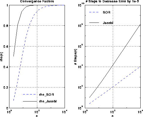
m ~ (n+1)/(2*pi)This is approximately the square root of the number of steps Jacobi requires. This is shown in the figures below.
A complexity analysis similar to that for Jacobi shows that
  Time(SOR)
      = number_of_steps * cost_per_step
      = O(sqrt(N)) * ( (N/p)*f + alpha + (n/p)*beta )
      = O(N^(3/2) /p)*f + O(sqrt(N))*alpha + O(N /p)*beta
where O(N/p) flops are needed to update local values,
alpha is the start up cost of messages to each neighbor, and
O(n/p) boundary values are communicated to neighbors.
     x = initial guess for inv(A)*b
     r = b - A*x   ... residual, to be made small
     p = r         ... initial "search direction"
     repeat
        v = A*p
            ... matrix-vector multiply
        a = ( r'*r ) / ( p'*v )
            ... dot product (BLAS1)
        x = x + a*p
            ... compute updated solution
            ... using saxpy (BLAS1)
        new_r = new_r - a*v
            ... compute updated residual
            ... using saxpy (BLAS1)
        g = ( new_r'*new_r ) / ( r'*r )
            ... dot product (BLAS1)
        p = new_r + g*p
            ... compute updated search direction
            ... using saxpy (BLAS1)
        r = new_r
     until ( new_r'*new_r small enough )
Here is a rough motivation for this algorithm. CG maintains
3 vectors at each step, the approximate solution x,
its residual r=A*x-b, and a
search direction p, which is also called a
conjugate gradient.
At each step x is improved by searching for a better solution
in the direction p, yielding an improved solution x+a*p.
This direction p is called a gradient because we are in fact doing
gradient descent on a certain measure of the error
(namely sqrt(r'*inv(A)*r)). The directions pi and pj from
steps i and j of the algorithm are called conjugate, or more
precisely A-conjugate, because they satisfy pi'*A*pj = 0 if i.ne.j.
One can also show that after i iterations
xi is the "optimal" solution among all possible linear
combinations of the form
a0*x + a1*(A*x) + a2*(A^2*x) + a3*(A^3*x) + ... + ai*(A^i*x)
For most matrices, the majority of work is in the sparse matrix-vector multiplication v=A*p in the first step. For Poisson's equation, where we can think of p and v living on a square grid, this means computing
     v(i,j) = 4*p(i,j) - p(i-1,j) - p(i+1,j)
                       - p(i,j-1) - p(i,j+1)
which is nearly identical to the inner loop of
Jacobi or SOR in the way it is parallelized.
We will deal with more general techniques for sparse-matrix-vector
multiplication in a later lecture.
The other operations in CG are easy to parallelize. The saxpy operations are embarrassingly parallel, and require no communication. The dot-products require local dot-products and then a global add using, say, a tree to form the sum in log(p) steps.
The rate of convergence of CG depends on a number kappa called the condition number of A. It is defined at the ratio of the largest to the smallest eigenvalue of A (and so is always at least 1). A roughly equivalent quantity is norm(inv(A))*norm(A), where the norm of a matrix is the magnitude of the largest entry. The larger the condition number, the slower the convergence. One can show that the number of CG iterations required to reduce the error by a constant g<1 is proportional to the square root of kappa. For Poissons's equation, kappa is O(N), so n=sqrt(N) iterations are needed. This means SOR and CG take about the same number of steps. An advantage of CG over SOR is that CG is applicable to a much larger class of problems.
There are methods similar to CG that are suitable for matrices A that are not symmetric or positive definite. Like CG, most of their work involves computing the matrix vector product A*p (or possibly A'*p), as well as dot-products and saxpy's. For on-line documenation and software, including advice on choosing a method, see "Templates for the Solution of Linear Systems".
We are going to rewrite the discrete Poisson equation as a slightly different matrix equation. To motivate it, consider the continuous Poisson equation
          d^2 u(x,y)   d^2 u(x,y)
          ---------- + ----------  = f(x,y)
            d x^2          d y^2
and discretize one derivative term at a time.
Then
          d^2 u(i*h,j*h)   U(i-1,j) - 2*U(i,j) + U(i+1,j)
          -------------- ~ ------------------------------
               d x^2                   h^2
Now consider the n-by-n matrix whose (i,j) entry is the right-hand-side of
the above equation. We claim that this matrix may be written as the
matrix-matrix product (-1/h^2)*T*U, where U is the n-by-n matrix of U(i,j)'s,
and T is the familiar symmetric tridiagonal matrix
              [  2  -1                 ]
              [ -1   2  -1             ]
          T = [     -1   2  -1         ]
              [       ... ... ...      ]
              [             -1  2  -1  ]
              [                -1   2  ]
A formal proof requires the simple computation:
  (T*U)(i,j) = sum_k T(i,k)*U(k,j)
             =  T(i,i-1)*U(i-1,j)
                + T(i,i)*U(i,j)
                + T(i,i+1)*U(i+1,j)
             = -U(i-1,j) + 2*U(i,j) - U(i+1,j)
since only 3 entries of row i of T are nonzero.
A completely analogous argument shows that
  d^2 u(i*h,j*h)   U(i-1,j) - 2*U(i,j) + U(i+1,j)
  -------------- ~ ------------------------------
       d x^2                   h^2

                   -1
                 = --- * (U*T)(i,j)
                   h^2
and so the Discrete Poisson equation may be written
T*U + U*T = Bwhere the (i,j)-th entry of B is b(i,j), as before.
Here is how we will solve T*U+U*T=B for U. Suppose we know how to factorize T = Q*Lambda*inv(Q), where Q is a known nonsingular matrix, inv(Q) is its inverse, and Lambda is a known diagonal matrix. (Later we will see that is simply another way to say that the columns of Q are eigenvectors of T and the diagonal entries of Lambda are eigenvalues. We will also write down explicit formulas for Q and Lambda.) Substituting this expression for T into T*U+U*T=B yields
(Q*Lambda*inv(Q))*U + U*(Q*Lambda*inv(Q)) = B .Now premultiply this equation by inv(Q) and postmultiply it by Q to get
Lambda*(inv(Q)*U*Q) + (inv(Q)*U*Q)*Lambda = inv(Q)*B*Qor, letting Ubar=inv(Q)*U*Q and Bbar=inv(Q)*B*Q,
Lambda*(Ubar) + (Ubar)*Lambda = Bbar .We want to solve this equation for Ubar, because then we can compute U=Q*Ubar*inv(Q). The (j,k)-th entry of this last equation is simple to evaluate, since Lambda is diagonal:
Lambda(j,j)*Ubar(j,k) + Ubar(j,k)*Lambda(k,k) = Bbar(j,k)We may now solve for Ubar(j,k) as follows:
Ubar(j,k) = Bbar(j,k)/(Lambda(j,j)+Lambda(k,k))This lets us state the overall high-level algorithm to solve T*U+U*T=B for U as follows:
  (1) Compute Bbar = inv(Q)*B*Q
  (2) For each j,k compute
         Ubar(j,k) = Bbar(j,k)/(Lambda(j,j)+Lambda(k,k))
  (3) Compute U = Q*Ubar*inv(Q)
Step (2) of this algorithm costs just 2*n^2=2*N operations,
and is embarrasingly parallel.
Steps (1) and (3) appear to cost 2 matrix-matrix multiplies
by Q and and 2 by inv(Q), for a cost of O(n^3)=O(N^(3/2)). This would
be no cheaper than SOR. But we will soon see
that Q is very special, so that in fact
Now we will go back and show how the factorization T = Q*Lambda*inv(Q) arises. Suppose q(j) is an eigenvector of T and lambda(j) is its corresponding eigenvalue. This means T*q(j) = lambda(j)*q(j). We can write this equation for j=1 to n as the following single matrix equation:
T*[ q(1), ... , q(n) ] = [ q(1)*lambda(1), ... , lambda(n)*q(n) ]or
T*Q = Q*Lambda ,where Q is a matrix whose columns q(j) are the eigenvectors:
Q = [q(1), q(2), ... q(n)]and Lambda is a diagonal matrix of eigenvalues
Lambda(j,j) = lambda(j) .Now, assuming Q is nonsingular, postmultiply T*Q = Q*Lambda by inv(Q) to get T=Q*Lambda*inv(Q) as desired.
It turns out we know an explicit expression for the eigenvalues lambda(i) and eigenvectors q(i) of T:
   lambda(j) = 2*(1-cos(j*pi/(n+1))

and

   Q(j,k) = sin(j*k*pi/(n+1)) * sqrt(2/(n+1)) = Q(k,j)       .
We will give an intuitive meaning to this expression in Lecture 20. In the meantime one can simply confirm that T*q(j) = lambda(j)*q(j) using elementary trigonometry.
Q has the further attractive property of being orthogonal, which means that its columns are orthogonal to one another and have unit length. This implies that inv(Q) = Q'=Q, and so
T = Q*Lambda*inv(Q) = Q*Lambda*Q .This lets us simplify our algorithm to
  (1) Compute Bbar = Q*B*Q
  (2) For each j,k compute
         Ubar(j,k) = Bbar(j,k)/(Lambda(j,j)+Lambda(k,k))
  (3) Compute U = Q*Ubar*Q
This makes it clear that all we need is a fast algorithm for multiplying
a matrix (or vector) by Q. To show how to do this, we first review the
FFT.
Definition. The Discrete Fourier Transform of an m-by-1 vector v is the matrix-vector product F*v, where F is an m-by-m matrix defined as follows. Let
omega = exp(2*pi*i/m) = cos(2*pi/m) + i*sin(2*pi/m),i.e. a complex number with absolute value 1, whose m-th power is 1 (a so-called m-th root of unity). Then for 0 <= j,k <= m-1, F(j,k) = omega^(j*k).
A standard fact about F is that inv(F) = complex_conjugate(F)/m, so that F/sqrt(m) is a unitary matrix (the complex equivalent of an orthogonal matrix). This means that multiplying by F and inverse(F) are essentially equivalent problems. (This can be confirmed by elementary trigonometry.)
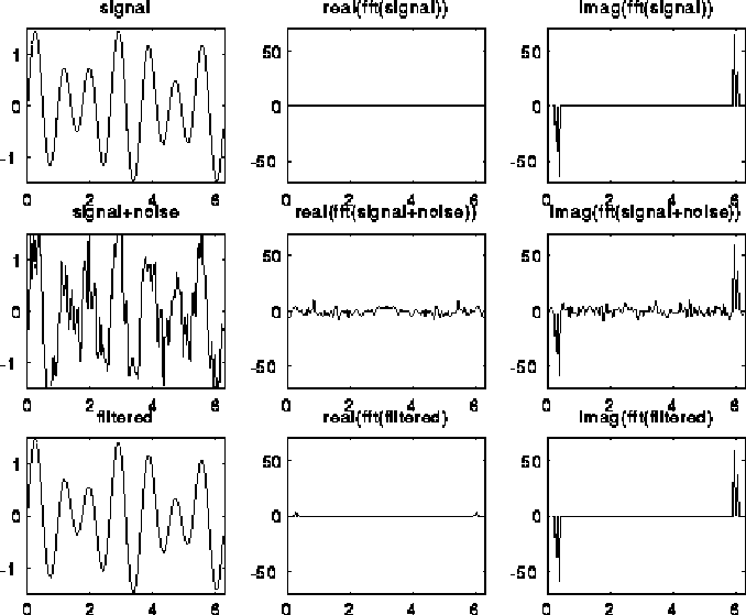
A typical use of the DFT is filtering, as illustrated below. The top left plot is the signal s=sin(7t)+.5*sin(5t), for t at 128 equally spaced points between 0 and 2*pi. The top right 2 plots are the real and imaginary part of the fft of the signal; there are essentially two pairs of spikes, corresponding to the two sine waves. The middle left plot is s with random noise added to it, which is bounded in magnitude by .75. Its fft is also shown to the right. Finally, the signal+noise is filtered by taking the fft of the signal+noise and zeroing out any components less than .25 in magnitude. This accurately restores the original signal, in the bottom left graph. More sophisticated filtering schemes are also used.
The Fast Fourier Transform (FFT) is an algorithm to compute the Discrete Fourier Transform F*v in O(m log m) time instead of O(m^2) time. We discuss it in more detail below, but first we will show how multiplying by F and multiplying by Q are closely related.
     F(j,k) = cos(2*pi*j*k/(2*(n+1))) + i * sin(2*pi*j*k/(2*(n+1)))
            = cos(pi*j*k/(n+1) + i * sin(pi*j*k/(n+1))
By comparing this expression with our earlier expression for Q,
Q(j,k) = sin((j+1)*(k+1)*pi/(n+1)) * sqrt(2/(n+1)) = Q(k,j) .we see that Q is the imaginary part of a submatrix of F
Q = Imag( F(1:n, 1:n) )(Imag(x) denotes the imaginary part of x). Thus, continuing to use Matlab notation, one can write
Q*v = Imag( ( F*vv )(1:n) ) where vv = [ 0; v; zeros(n,1) ]In other words, we could extend v with one 0 at the top and n zeros at the bottom to get vv, do a 2*(n+1) point FFT on vv to get F*vv, and extract the imaginary part of components 1 through n from components 0 through 2*n+1 of F*vv. Matlab code for a function fast_sine_transform(V) which performs Q*V for a matrix V is as follows (note that it uses Matlab's built-in fft function).
     % Fast Sine Transform on input matrix V
     % of dimension n-by-m
     function Y=fast_sine_transform(V)
     [n,m]=size(V);
     V1=[zeros(1,m);V;zeros(n+1,m)];
     V2=imag(fft(V1));
     % In Matlab vectors and matrices are indexed
     % starting at 1, not 0
     Y=V2(2:n+1,:);
Using fast_sine_transform, a Matlab implementation of the entire FFT-based Poisson solver is
    % Solve the discrete Poisson equation
    % on an n-by-n grid with right hand side b
    function X=Poisson_FFT(B)
    [n,m]=size(b);
    % Form eigenvalues of matrix T(nxn)
    L=2*(1-cos((1:n)*pi/(n+1)));
    % Form reciprocal sums of eigenvalues
    % Include scale factor 2/(n+1)
    LL=(2/(n+1))*ones(n,n)./(L'*ones(1,n)+ones(n,1)*L);
    % Solve, using the Fast Sine Transform
    X = fast_sine_transform(b');
    X = fast_sine_transform(X');
    X = LL.*X;
    X = fast_sine_transform(X');
    X = fast_sine_transform(X');
In practice, one can multiply by Q quickly (by a constant factor)
without using the complex FFT, but rather another
divide-and-conquer algorithm
very similar to the one described below.
Much software for this and related problems is available on
Netlib, in the subdirectories
We begin by showing how to interpret the product F*v as polynomial evaluation of the polynomial
V(x) = sum_{k=0}^{m-1} x^k * v(k)
at the points x = omega^0, omega^1, omega^2, ..., omega^(m-1):
     (F*v)(j) = sum_{k=0}^{m-1} F(j,k) * v(k)
              = sum_{k=0}^{m-1} omega^(j*k) * v(k)
              = sum_{k=0}^{m-1} (omega^j)^k * v(k)
              = V(omega^j)
Conversely, one can interpret multiplication by inv(F) as
polynomial interpolation, i.e. computing the coefficients of
a polynomial given its value at m points omega^j.
Now break up the polynomial V(x) into two parts, those consisting of even powers of x, and those consisting of odd powers of x:
      V(x) = v(0) + x^2 * v(2) + x^4 * v(4) + ...
                  + x^1 * v(1) + x^3 * v(3) + ...
           = (v(0) + x^2 * v(2) + x^4 * v(4) + ...)
             + x * (v(1) + x^2 * v(3) + x^4 * v(5) + ...)
(*)        = V_even(x^2) + x * V_odd(x^2)
Since V is a polynomial of degree m-1, V_even and V_odd are polynomials
of degree m/2 - 1, which we need to evaluate at the points
(omega^j)^2, for 0 <= j <= m-1. But this is really just (m/2) different
points omega^(2*j) for 0 <= j <= (m/2)-1 since
    (omega^(j+m/2))^2
        = (omega^j * omega^(m/2))^2
        = (omega^j)^2 * omega^m
        = (omega^j)^2
          ... since omega^m = 1 by construction
Thus, evaluating V(x) at m values omega^j is equivalent to evaluating
two half sized problems (V_odd and V_even at half as many points),
and then combining their values in a simple way. This leads to the
following recursive, divide-and-conquer algorithm for the FFT:
  function x = FFT(v,omega,m)
     if m=1 then
        return v(0)
     else
        v_even = FFT(v(0:2:m-2), omega^2, m/2)
                 ... v(0:2:m-2) = v(0,2,4,...,m-2)

        v_odd  = FFT(v(1:2:m-1), omega^2, m/2)
                 ... v(1:2:m-1) = v(1,3,5,...,m-1)

        omegav = [ omega^0, omega^1, omega^2, ... ,
                   omega^((m/2)-1) ]
                 ... in practice these coefficients are
                 ... precomputed and stored in a table

        return x = [v_even + ( omegav .* v_odd ),
                    v_even - ( omegav .* v_odd )]
                 ...  omegav .* v_odd is the component-wise
                 ...  product of these two vectors
     end if
The reason for using +omegav.*v_odd and -omegav.*v_odd is that when
x = omega^(j+(m/2)) in equation (*) above,
omega^(j+(m/2)) = omega^j * omega^(m/2) = -omega*j
We compute the complexity of this algorithm as follows. Let FFT_time(m) be the cost of the algorithm on an input of size m. Then from the structure of the algorithm
FFT_time(m) = 2 * FFT_time(m/2) + O(m)where 2*FFT_time(m/2) is the cost of the two recursive calls, and O(m) is the cost of m/2 products, sums and differences in computing x. Change variables to s = log_2 m to get
FFT_time(s) = 2 * FFT_time(s-1) + O(2^s)
This simple recurrence has the value FFT_time(s) = O(2^s) + O(2^s) + ... O(2^s) (s terms), or O(s*2^s) = O(m log m), as desired.
It is not necessary for m to be a power of 2 to use the divide-and-conquer technique in this algorithm. Indeed, Gauss first invented this algorithm for m=12 centuries ago. To be efficient, m should be a product of many small prime factors.
                                             F( 0,1,2,...,15 )
                                             = F( xxxx_2 )
                                               |        |
                          ----------------------        -----------------------
                          |                                                   |
                   F( even )                                                 F( odd )
                   = F( 0,2,4,...,14)                                        = F( 1,3,5,...,15 )
                   = F( xxx0_2 )                                             = F( xxx1_2 )
                     |       |                                                  |      |
           -----------       ------------                             -----------      -------------
           |                            |                             |                             |
     F( 0,4,8,12 )                F( 2,6,10,14 )                F( 1,5,9,13 )                 F( 3,7,11,15 )
     = F( xx00_2 )                = F( xx10_2 )                 = F( xx01_2 )                 = F( xx11_2 )
         |   |                         |   |                         |   |                          |   |
    ------   -------              ------   -------              ------   -------              -------   --------
    |              |              |              |              |              |              |                |
F( 0,8 )       F( 4,12 )      F( 2,10 )      F( 6,14 )      F( 1,9 )       F( 5,13 )      F( 3,11 )        F( 7,15 )
= F( x000_2 )  = F( x100_2 )  = F( x010_2 )  = F( x110_2 )  = F( x001_2 )  = F( x101_2 )  = F( x011_2 )    = F( x111_2 )
 |       |       |      |      |       |      |       |      |        |     |       |      |       |        |       |
 |       |       |      |      |       |      |       |      |        |     |       |      |       |        |       |
F(0)    F(8)    F(4)   F(12)  F(2)    F(10)  F(6)    F(14)  F(1)     F(9)  F(5)    F(13)  F(3)    F(11)    F(7)    F(15)
0000    1000    0100   1100   0010    1010   0110    1110   0001     1001  0101    1101   0011    1011     0111    1111
Practical FFT algorithms are not recursive, but iterative. The iterative implementation loops across each level of the tree illustrated above, beginning at the leaves, and moving toward the root. Note that at the bottommost level, we combine pairs of values whose bit patterns differ in the leftmost bit (for example 0 and 8, 4 and 12, 2 and 10, etc.) At the next level, we combine pairs of values whose bit patterns differ in the next-to-leftmost bit (eg 0 and 4, 8 and 12, 2 and 6, 10 and 14, etc.) This leads to the following algorithm. We use the notation k=k(0)k(1)...k(s-2)_2 to mean the binary representation of the (s-1)-bit integer k; each k(j) is either 0 or 1.
  for j = 0 to s-1     ... for each level of the call tree
                       ... from bottom to top

      for  k = 0 to (m/2)-1     ... for each vector entry

           t0 = v[k(0)k(1)...k(j-1)0k(j)...k(s-2)]
                       ... the subscript is equal to k with
                       ... 0 inserted before bit j

           t1 = v[k(0)k(1)...k(j-1)1k(j)...k(s-2)]
                       ... the subscript is equal to k with
                       ... 1 inserted before bit j

           w = omega^[0k(j-1)...k(0)0...0]
                       ... a power of omega stored in a table

           x = w.*t1   ... componentwise multiplication

           v[k(0)k(1)...k(j-1)0k(j)...k(s-2)] = t0 + x
                       ... update location of v containing t0

           v[k(0)k(1)...k(j-1)1k(j)...k(s-2)] = t0 - x
                       ... update location of v containing t1
      end for
  end for
The algorithm corresponds to the recursive version because setting the
j-th bit of a subscript to 0 is equivalent to taking the even subset of
subscripts, and setting the j-th bit to 1 is equivalent to taking the
odd subset.
The algorithm overwrites the input vector v with a permutation of the answer F*v. The permutation is called the bit-reverse permutation; component
k = k(0)k(1)...k(s-2)k(s-1)_2of the output vector contains component
reverse(k) = k(s-1)k(s-2)...k(2)k(0)_2of F*v.
Here is another, equivalent way to see the pattern of which components of v get combined with which other components at each step of the algorithm. As before, we illustrate in the case m = 2^4 = 16. Then we may partially evaluate the algorithm to see that
 When j=0          When j=1         When j=2         When j=3
   When k=0          When k=0         When k=0         When k=0
     t0 = v[0000]     t0 = v[0000]     t0 = v[0000]     t0 = v[0000]
     t1 = v[1000]     t1 = v[0100]     t1 = v[0010]     t1 = v[0001]
   When k=1          When k=1         When k=1         When k=1
     t0 = v[0001]     t0 = v[0001]     t0 = v[0001]     t0 = v[0010]
     t1 = v[1001]     t1 = v[0101]     t1 = v[0011]     t1 = v[0011]
   When k=2          When k=2         When k=2         When k=2
     t0 = v[0010]     t0 = v[0010]     t0 = v[0100]     t0 = v[0100]
     t1 = v[1010]     t1 = v[0110]     t1 = v[0110]     t1 = v[0101]
   When k=3          When k=3         When k=3         When k=3
     t0 = v[0011]     t0 = v[0011]     t0 = v[0101]     t0 = v[0110]
     t1 = v[1011]     t1 = v[0111]     t1 = v[0111]     t1 = v[0111]
   When k=4          When k=4         When k=4         When k=4
     t0 = v[0100]     t0 = v[1000]     t0 = v[1000]     t0 = v[1000]
     t1 = v[1100]     t1 = v[1100]     t1 = v[1010]     t1 = v[1001]
   When k=5          When k=5         When k=5         When k=5
     t0 = v[0101]     t0 = v[1001]     t0 = v[1001]     t0 = v[1010]
     t1 = v[1101]     t1 = v[1101]     t1 = v[1011]     t1 = v[1011]
   When k=6          When k=6         When k=6         When k=6
     t0 = v[0110]     t0 = v[1010]     t0 = v[1100]     t0 = v[1100]
     t1 = v[1110]     t1 = v[1110]     t1 = v[1110]     t1 = v[1101]
   When k=7          When k=7         When k=7         When k=7
     t0 = v[0111]     t0 = v[1011]     t0 = v[1101]     t0 = v[1110]
     t1 = v[1111]     t1 = v[1111]     t1 = v[1111]     t1 = v[1111]
There is an edge from a grid point v0 in column j to a grid point v1 in column j+1, if the data at v1 depends on the data at v0. From examining the algorithm, we see that there is an edge from both grid points
     [k(0)k(1)...k(j-1)0k(j)...k(s-2)]  and
     [k(0)k(1)...k(j-1)1k(j)...k(s-2)]  in column j
to the same grid points points in column j+1, for a total of 4 edges
connecting this pair of points.
These 4 edges form what looks like a "butterfly" in the figure below,
where we have color-coded the edges so that edges corresponding to the
same butterfly connecting adjacent columns have the same color.
Here is the graph in the case m=16. The first column of butterflies
connects grid points whose numbers differ in bit 0 (the leftmost bit).
For example, the black butterfly connects 0000 and 1000. The second
column of butterflies connects grid points whose numbers differ in bit 1;
for example the black butterfly connects 0000 and 0100.
The next black butterfly connect 0000 and 0010, and the rightmost black
butterfly connects 0000 and 0001.
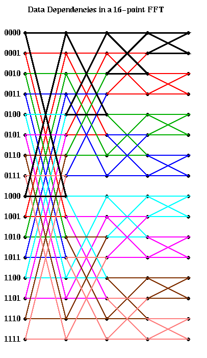
This analysis is enough to compute the PRAM complexity of the FFT: Each of the s rightmost columns can be computed in one time step using m processors, for a complexity of O(s) = O(log m).
For a real parallel implementation, we need to take communication costs into account, and this is dictated by our choice of layout: which processors own which entries of the vector v. The following discussion may be found in "LogP: Towards a realistic model of parallel computation", by D. Culler, R. Karp, D. Patterson et al, which is in the class reader.
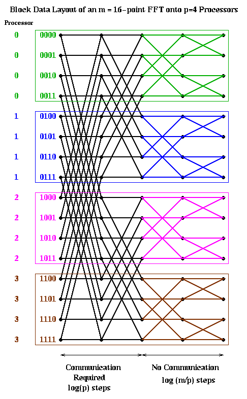
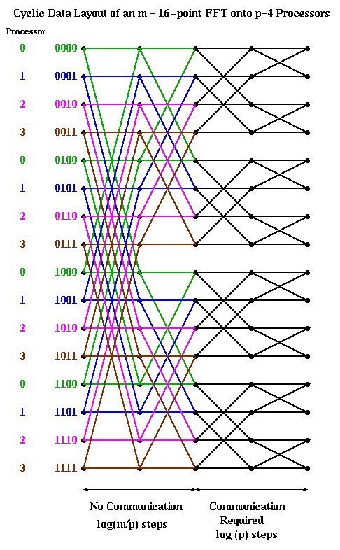
Let us consider two obvious candidates which we considered before in the case of Gaussian elimination: blocked and cyclic. The block case is shown below, with m=16 and p=4. The processor numbers are color coded. Edges which cross processor boundaries, and so require communication, are black. Edges within a processor, which require no communication, are color coded by the local processor color. In the block case, note that the leading log(p) bits of an address determine the processor (green is processor 00, blue is 01, magenta is 10, and brown is 11). Thus, in general, the first log(p) stages require communication, because addresses of data to be combined differ in their leading log(p) bits. The last log(m/p) stages are local, and require no communication.
The cyclic case is shown below, color coded in the same way. In this case, the trailing log(p) bits of an address determine the processor. Therefore, the last log(p) stages require communication, and the first log(m/p) stages are local.
Let us analyze the parallel complexity of these algorithms. As before we use the parameters.
     p = number of processors
     f = time per flop
     alpha = startup for a message
     beta = time per word in a message
Then both the block and cyclic implementations require
  Time(block_FFT) = Time(cylic_FFT) =
         2*m*log(m)/p * f     ... 2*m/p flops at log(m) stages
        + log(p) * alpha      ... one message per processor per
                              ... stage for log(p) stages
        + m*log(p)/p * beta   ... m/p words per message
An alternative implementation is start with a cyclic implementation, and then transpose the data to have a block layout after the first log(p) steps. This way the first log(p) stages require no communication, then a transpose (a significant amount of communication) is performed, and finally the last log(m/p) stages are again local. (This assumes m>=p^2, which we now assume, since we expect many more points than processors. Otherwise, there may be more transposes required.) This is shown below.
   1) perform "local FFTs"
   2) transpose
   3) perform "local FFTs"
(The "local FFTs" have the same structure as an FFT, but may use different powers of omega as coefficients.)
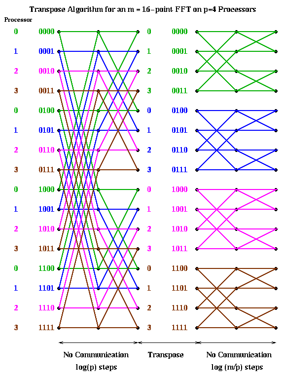
The reason we call converting from cyclic to block layout (or back) transposing is shown below for m=16 and p=4. When the data layout is seen in this way, it clearly looks like transposing a matrix.
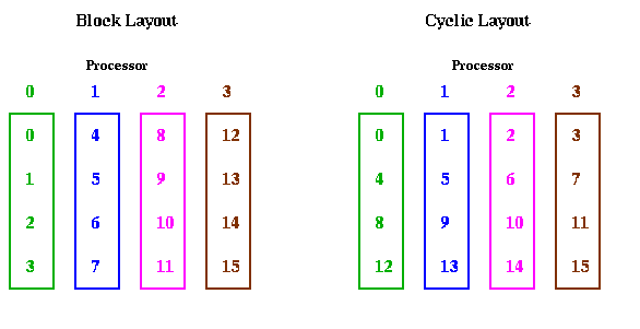
The computational cost of this algorithm is the same as before: 2*m*log(m)/p*f. The communication cost is entirely the cost of transposing a matrix. This in turn depends on details of how many messages can be overlapped in the network. In the most pessimistic case, where no communication can overlap, so a processor can have only one outstanding message to another processor at a time, the cost is as follows:
  Time(transpose_FFT) (non-overlapped) =
       = 2*m*log(m)/p * f       ... 2*m/p flops at log(m) stages
        + (p-1) * alpha         ... p-1 messages per processor
                                ... to transpose
        + m*(p-1)/p^2 * beta    ... m/p^2 words per message
Comparing Time(transpose_FFT) with Time(block_FFT) = Time(cyclic_FFT),
we see that the transpose_FFT sends less data overall, but sends
(p-1)/log p times as many messages. Thus, in this non-overlapping case,
one expects the transpose_FFT to do well in a low latency, high bandwidth
environment, or when m is very large and p small,
and the block or cyclic to do well
in a high latency, low bandwidth environment, or when m is not as large
but p is large.
In the most optimistic situation, where the communication hardware and software permit communications to overlap so that one can have many messages to other processors outstanding at a time, one pays only a latency cost of alpha, rather than p-1 alpha. This lowers the cost to
  Time(transpose_FFT) (overlapping) =
       = 2*m*log(m)/p * f       ... 2*m/p flops at log(m) stages
        + alpha                 ... p-1 overlapping messages
                                ... per processor to transpose
        + m*(p-1)/p^2 * beta    ... m/p^2 words per message
which is always better than either cylic_FFT or block_FFT.
In fact, one can show it is close to optimal
(see
"LogP: Towards a realistic model of parallel computation" for details).
The above algorithm does not attempt to return the answer in sorted order; it comes out in a permuted order, which is adequrate for many applications. Sorting the final answer would require more communication (essentially another transpose).
For a radically different way to parallelize the 1D FFT, which uses the Fast Multipole Method to lower the communication needed when one insists on sorted inputs and outputs, see the paper The Future Fast Fourier Transform? on Alan Edelman's homepage. See Lecture 24 and especially Lecture 25 for detail on the Fast Multipole Method.
There are three obvious algorithm and layout choices that one might consider for the 2D case:
2D Blocked Layout
Assume we are given the n-by-n grid of data in a 2D blocked layout, using an s-by-s processor grid, where s = sqrt(p). Thus, each processor owns an n/s-by-n/s subgrid, as shown below.
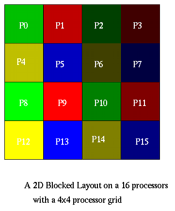
The algorithm is now easy to describe. Let N=n2. We first do 1D FFTs on all the rows using the 1D parallel FFT algorithm from above. In these row FFTs, s processors cooperate to solve each row, e.g., P0, P1, P2, and P3 solve the first n/s rows in the picture. The other processors proceed in parallel, so there total running time is that of n/s 1D FFTs of size n on s processors.
  Time(RowFFT) =
       O((n*log(n)/s)) * (n/s) * f  ... O(n*log(n)/s) flops per FFT
                                    ... times n/s FFTs
        + x*alpha                   ... s-1 messages per processor
                                    ... to transpose
                                    ... x=1 for overlap
                                    ... x=s-1 for no overlap
        + n^2*(s-1)/s^3 * beta      ... (n/s^2)*(n/s) words per message

       = O(N*log N / p)*f + x*alpha + N*((s-1)/s)/p *beta
where x=1 if all messages can overlap, and x=s-1=sqrt(p)-1 if they cannot
overlap.
The column FFTs have the same cost, and unlike some of the other strategies described below, no global redistribution of data is required. (Note that, depending on 2D array layout, one of the dimensions will not have stride one accesses, even at the bottom of the FFT butterfly.)
The total cost is therefore Time(RowFFT)+Time(ColumnFFT) = 2*Time(RowFFT) shown above.
Block Row Layout with Transpose
There is another much simpler implementation of this algorithm, which does not require parallelizing the FFT at all. If one can in fact fully overlap the latency cost of transposition, its cost is identical to the algorithm above. In the somewhat more general and realistic situation of nonoverlapping communication, it costs the same in flops and bandwidth, and sqrt(p) times as much in latency:
  1) Layout out the data by block row
     (processor i gets rows i*(n/p) through (i+1)*(n/p)-1)
  2) Perform FFTs on locally stored n/p rows. These require
     no communication.
  3) Transpose the data, so processor i gets columns i*(n/p) through
     (i+1)*(n/p)-1) instead of rows
  4) Perform FFTs on local n/p columns. These again require no
     communication.
The cost of this is
   O((n*log(n)) * (n/p) * f   ... O(n*log(n)) flops per FFT
                              ... times n/p FFTs
    + x*alpha                 ... p-1 messages per processor
                              ... to transpose
                              ... x=1 for overlap
                              ... x=p-1 for no overlap
    + n^2*(p-1)/p^2 * beta    ... (n^2/p^2) words per message

   = O(N*log N / p)*f + x*alpha + N*((p-1)/p)/p *beta
Block Row Layout without a Transpose
Another alternative is to use the block row layout above, but to leave the data in this layout for the column FFTs. In this case, the column FFTs will be 1D parallel FFTs, each on p processors. We avoid the transpose at the cost of more expensive 1D FFTs.
For more details, including comparisons of some of these models to actual measurements, see "Performance Modeling and Composition: A Case Study in Cell Simulation" by S. Steinberg, J. Yang, and K. Yelick. This paper actually uses the parallel solution of Poisson's equation as one step in a more complicated problem involving simulating the motion of biological cells immersed in moving fluids. These techniques have been used to study blood flow in the heart, embryo growth, platelet aggregation in blood clotting, sperm motility, and other biological processes.
The 3D case
As mentioned ealier, the 3D case is entirely analogous to the 2D. One can imagine using a 3D blocked layout on a c x c x c processor grid (where c = p1/3). Note that the three dimensions need not be identical for the algorithm to work correctly. Alternatively, each processor could own complete planes, so the FFTs in 2 dimensions would require no communication; the 3rd dimension could be acheived with either a tranpose or a parallel 1D FFT.