We will show how to implement matrix multiplication C=C+A*B on several of the communication networks discussed in the last lecture, and develop performance models to predict how long they take. We will see that the performance depends on several factors.
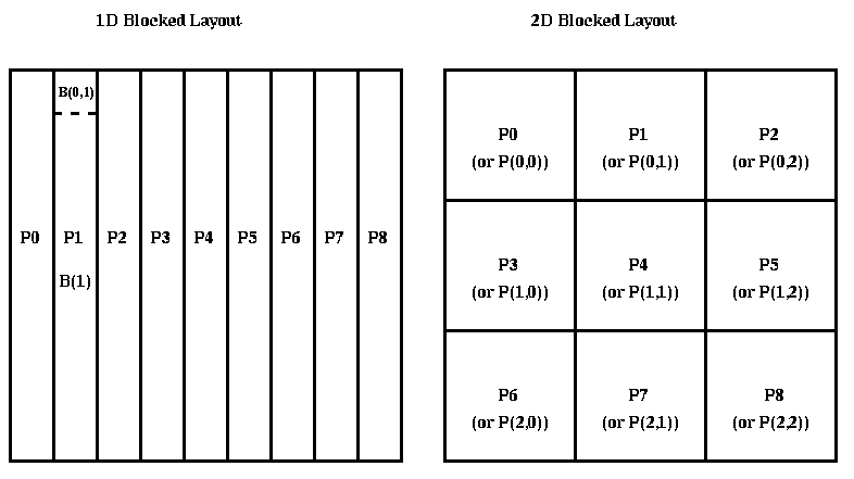
We will begin by examining the 1D Blocked Layout on a bus without broadcast (like a single ethernet), a bus with broadcast, and a ring of processors.
The algorithm depends on the following simple formula from linear algebra:
C(i) = C(i) + A*B(i) = C(i) + sum_{j=0}^{p-1} A(j)*B(j,i)
Since processor i owns C(i) and B(i), but not each A(j) as required by the
formula, the algorithm will have to send each A(j) to each processor.
This is similar to the Sharks and Fish 2 problem, fish moving under gravity,
where each fish (A(j)) has to visit each processor in order to perform
the computation.
Our first model of a bus is that at most one processor may send, and at most one may receive at a time. A floating point operation costs 1 time unit, message startup costs alpha time units, and the cost per work is beta time units. In other words, sending a message of n words takes alpha + beta*n time units. We use synchronous send and receive.
Here is the algorithm:
  Matrix multiplication with a 1D blocked layout on a bus
    without broadcast, and with a barrier.

  C(MYPROC) = C(MYPROC) + A(MYPROC)*B(MYPROC,MYPROC)
  for i=0 to p-1
     for j=0 to p-1 except i
        if ( MYPROC = i ) send A(i) to processor j
        if ( MYPROC = j )
           receive A(i) from processor i
           C(MYPROC) = C(MYPROC) + A(i)*B(i,MYPROC)
        endif
        barrier()
     end for
  end for
The cost of the arithmetic in the inner loop is 2*n*(n/p)^2 = 2*n^3/p^2,
and the cost of the communication in the inner loop is alpha + n*(n/p)*beta,
so the overall time is
   Time = (p*(p-1)+1)*(2*n^3/p^2)             ... arithmetic
          + (p*(p-1))*( alpha + n*(n/p)*beta) ... communication

        ~ 2*n^3 + p^2*alpha + p*n^2*beta
where we have ignored lower order terms in p in the second formula.
This is more than the serial time, 2*n^3, and grows with p rather than
shrinking with p, and so is a rather poor parallel algorithm!
In fact, it is not really parallel at all, since at most processor
can compute at a time, because of the barrier.
So we can hope to do better by removing the barrier, in order to overlap computation and communication, and to send A(i) to several processors so they can operate in parallel. Here is the algorithm without a barrier:
  Matrix multiplication with a 1D blocked layout on a bus
    without broadcast, and without a barrier.

  C(MYPROC) = C(MYPROC) + A(MYPROC)*B(MYPROC,MYPROC)
  for i=0 to MYPROC-1
      receive A(i) from processor i
      C(MYPROC) = C(MYPROC) + A(i)*B(i,MYPROC)
  end for
  for i=0 to p-1 except MYPROC
      send A(MYPROC) to processor i
  end for
  for i=MYPROC+1 to p-1
      receive A(i) from processor i
      C(MYPROC) = C(MYPROC) + A(i)*B(i,MYPROC)
  end for
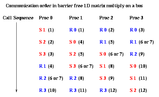
This program is non-deterministic, in the sense
that the sends and receives in the algorithm without a barrier do not
necessarily have to occur in the same order as the algorithm with a barrier.
For example, the following figure shows the sequence in which sends and
receives occur when there are 4 processors. There is one column for
each processor, containing the sends and receives in the order each
processor calls them; Sj means "send to proc j" and Ri means "receive
from proc i". Each send and receive is labeled by the order in which
it occurs. For example, "S2 (5)" in the column for processor 1
and "R1 (5)" in the column for processor 2
means that the fifth communication involves processor 1 sending to
processor 2. Note that the two communications from processor 1 to 3, and from
processor 2 to 0, may occur in either order (either may occur sixth or
seventh).
(Technically, we say the partial orders imposed on the communication
events by the p programs on each processor do not constitute a
total order.)
This race condition is not important, because the same results are computed
no matter what the order is.
Let us analyze the performance of this algorithm. Intuitively, if the cost of a communication step,
cm = alpha + n*(n/p)*beta,is sufficiently smaller than the cost of arithmetic in the inner loop,
ar = 2*n^3/p^2,then efficiency should be high. Conversely, if communication is comparable to, or dominates, computation, we expect low efficiency. If we keep p fixed and let n grow, then since ar grows like n^3 and cm like n^2, we expect ar to dominate cm for large enough problems, and high efficiency to be achieved.
Now we will quantify this intuition. Let us draw the time-line for this algorithm, assuming that cm <= ar. In the time-line, a block of time labeled i->j refers to communication from processor i to j and takes time cm, and a block of time labeled jC refers to processor j computing, and takes time ar. For simplicity we assume communications occur in the same order as the program with a barrier, although as stated above this should not matter.
  time --->
  |   0C   |
  |   1C   |
     ...
  |   p-1C |
           | 0->1 |   1C   |
                  | 0->2 |   2C   |
                         | 0->3 |   3C   |
                                ...
                                    |0->p-1| p-1C   |
                                             ...
As shown in the diagram, the overall computation forms a pipeline.
To compute the duration of the pipeline, we need to consider whether
there are any "bubbles" in the pipeline, i.e. if the communication
steps cannot happen without intervening delays.
In particular, the next communication to follow 0->p-1 is 1->0. 1->0 will
be able to start without delay after 0->p-1 completes provided processor
1 is not busy, i.e. provided computation 1C has completed. This will be the
case if ar <= (p-2)*cm, in which case the total time is
Time = p*(p-1)*cm + 2*arUsing the inequality ar <= (p-2)*cm and some algebra yields
2*n^3/p = p*ar < Time <= (p^2+p-4)*cmThe lower bound 2*n^3/p is (nearly) attained when cm equals its lower bound ar/(p-2). This corresponds to (nearly) perfect speedup, since the serial time is 2*n^3. Thus, if communication is so fast that cm ~ ar/(p-2), the fact that the bus is a serial bottleneck does not matter. If cm is even smaller than ar/(p-2), so there are "bubbles" in the pipeline, the speedup can improve a little, but not much.
As cm grows, the speedup shrinks. When cm=ar, the running time is (p^2-p+2)*ar ~ 2*n^3, or approximately equal to the serial running time. In other words, parallelism does not help at all. If cm is larger than ar, the running time is slower than the serial algorithm. These possibilities are captured in the efficiency formula
      Efficiency = Serial_Time / ( p * Parallel_Time )
                 = 1 / ( 2/p + (p-1)*cm/ar )
                 = 1 / ( 2/p + (p^3-p^2)/(2*n^3)*alpha
                             + (p^2-p)/(2*n)*beta )
and we are assuming 1/(p-2) <= cm/ar <= 1.
When cm/ar is close to 1/(p-2), efficiency
is near 1. When cm/ar is close to 1, efficiency is nearly 1/p, i.e. there
is no speedup at all.
From the expression for n/p, we see that cm/ar is small when n>>p, and when
alpha and beta are not too large. One could easily plug in particular values
of n, p, alpha and beta to measure the efficiency for a particular
matrix size on a particular machine.
Here is the algorithm:
  Matrix multiplication with a 1D blocked layout on a bus
     with broadcast and no barrier.

  C(MYPROC) = C(MYPROC) + A(MYPROC)*B(MYPROC,MYPROC)
  for i=0 to p-1
     if ( MYPROC = i )
        broadcast A(i)
     else
        receive A(i) from processor i
     endif
     C(MYPROC) = C(MYPROC) + A(i)*B(i,MYPROC)
  end for
Assuming the same communication model, the time is now
   Time =  p*2*n^3/p^2 + p*( alpha + n^2/p*beta )
        = 2*n^3/p + p*alpha + n^2*beta
so
      Efficiency = Serial_Time / ( p * Parallel_Time )
                 = 1 / ( 1 + cm/ar )
                 = 1 / ( 1 +
                         p^2/(2*n^3)*alpha +
                         p/(2*n)*beta )
In contrast to the bus without broadcast, the cm/ar term in the
denominator of the efficiency is p-1 times smaller, and so efficiency is
a much less sensitive function of p.
As before, since we expect alpha>>1 and beta>>1, we require n>>p for
parallelism to be effective. However, since there is p times less communication
time, our lower bound on n/p for effective parallelism is much lower than
for a bus without broadcast, quantifying our intuition that more
communication helps parallelism.
  Matrix multiplication with a 1D blocked layout on a ring

  copy A(MYPROC) into T
  C(MYPROC) = C(MYPROC) + T*B(MYPROC,MYPROC)
  for i=1 to p-1
     send T to processor MYPROC+1 mod p
     receive T from processor MYPROC-1 mod p
     C(MYPROC) = C(MYPROC) + T * B( (MYPROC-i) mod p, MYPROC )
  end for
Assuming the same communication model, the time is now
   Time = p*2*n^3/p^2 + (p-1)*( alpha + n^2/p*beta )
        = 2*n^3/p + (p-1)*alpha + (p-1)/p * n^2*beta
and the efficiency is
   Efficiency = 1 / ( 1 + (p-1)/p * cm/ar )
              = 1 / ( 1 +
                     p*(p-1)/(2*n^3)*alpha +
                     (p-1)/(2*n)*beta )
which is just slightly faster than the time for the broadcast bus.
It is easy to see that this is essentially optimal, for a 1D blocked layout on a bus or ring, because the matrix multiplication formula we use requires every product A(i)*B(i,j) to eventually accumulate on processor j, which entails some data of size n*(n/p) moving from each processor i to each processor j, and this requires at least p-1 messages of size n^2/p.
Since a ring may be embedded in a mesh or hypercube, the same algorithm also works on these networks. But as we will see, much better algorithms are available.
Cannon's algorithm reorders the summation in the inner loop of block matrix multiplication as follows:
   C(i,j) = C(i,j) + sum_{k=0}^{s-1} A(i,k)*B(k,j)
          = C(i,j) + sum_{k=0}^{s-1} A(i, (i+j+k) mod s)*B( (i+j+k) mod s, j)
   Cannon's matrix multiplication algorithm

   for all (i=0 to s-1)      ...  "skew" A
      Left-circular-shift row i of A by i,
          so that A(i,j) is overwritten by A(i, (j+i) mod s)
   end for
   for all (i=0 to s-1)      ... "skew" B
      Up-circular-shift column i of B by i,
          so that B(i,j) is overwritten by B( (i+j) mod s, j)

   end for
   for k=0 to s-1
      for all (i=0 to s-1, j=0 to s-1)
          C(i,j) = C(i,j) + A(i,j)*B(i,j)
          Left-circular-shift each row of A by 1,
              so that A(i,j) is overwritten by A(i, (j+1) mod s)
          Up-circular-shift each column of B by 1,
              so that B(i,j) is overwritten by B( (i+1) mod s, j)
      end for
   end for
The following picture illustrates the algorithm for 9 processors:
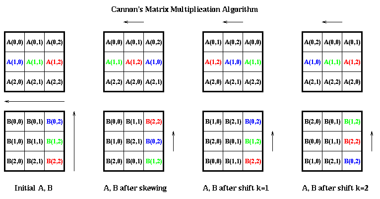
In other words, after the initial "skewing", each data movement A(i,k) and B(k,j) arrive at processor P(i,j), and are multiplied and accumulated into C(i,j). The k's occur in different permutations on different processors, as described by (i+j+k) mod s.
For example, in the picture above the 3 colored blocks are accumulated to form C(1,2). First the blue blocks A(1,0) and B(0,2) are co-resident in P(1,2) and multiplied and accumulated. Then the green blocks A(1,1) and B(1,2) are multiplied and accumulated, and finally the red blocks A(1,2) and B(2,2) are multiplied and accumulated.
This algorithm is well suited to an s-by-s mesh of processors, for which we will now measure the performance.
The total cost is thereforeTime = 2*n^3/p + 3*sqrt(p)*alpha + 3*n^2/sqrt(p) * betawith efficiency
    Efficiency = 1 / ( 1 +
                       1.5*p^(1.5)/n^3*alpha +
                       1.5*p^(.5)/n*beta )
Comparing with the time for a ring, we see the arithmetic time is the
same, but the communication time is about sqrt(p) times smaller. This
reflects the fact that the bisection width of a mesh is sqrt(p) times
as large as a ring.
C(i,j) = C(i,j) + sum_{k=0}^{s-1} A(i,k)*B(k,j)
be done by processor (i,j,k) in the 3D mesh. Then the sums are accumulated
along rows of the mesh. See
"A three-dimensional approach to parallel matrix multiplication"by
R. Agarwal et al, IBM J. of Res. and Dev., v. 39, n. 5, pp 521-600,
Sept. 1995. for details.
We will first show how to map Cannon's algorithm to a hypercube, and then how to speed it up. Recall from the last lecture how we map a 2D mesh to a hypercube. Suppose the mesh is 2^m-by-2^m, where 2^m = s. Let G(m) = { g(0), ... , g(2^m-1) } be the m-bit Gray code. Then processor (i,j) in the mesh is mapped to processor g(i)*2^m+g(j) in the hypercube. In other words, we just concatenate the m bits in g(i) and the m bits in g(j) to get the hypercube address. An example for m=2 is shown below. Students of digital design will recognize that this is the same idea as a Karnaugh map.
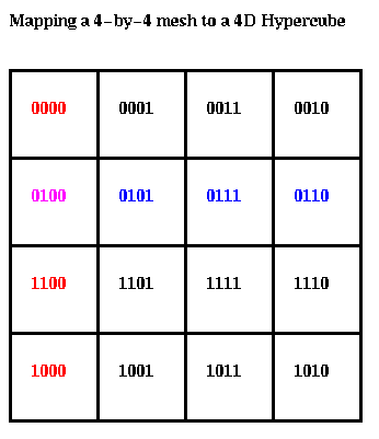
This mapping makes it clear that columns of the matrix are mapped to independent sub-hypercubes of the original hypercube, and the same for columns. For example, the blue column above is mapped into the blue sub-hypercube below, and the same for the red row and red sub-hypercube.
Thus, we can use the more numerous wires of the hypercube to accelerate the skewing phase of Cannon's algorithm. This variation is due to Dekel, Nassimi and Sahni. We assume without loss of generality that A(i,j) is stored on processor i*2^m + j.
  Dekel, Nassimi and Sahni's hypercube matrix multiply

  for k= 0 to m-1
      jk = 2^k and j  ... "logical and" of 2^k and j
      ik = 2^k and i  ... "logical and" of 2^k and j
      for all (i=0 to s-1, j=0 to s-1)
          swap A(i, j xor ik) and A(i, j)   ... "exclusive or" of j and jk
          swap B(jk xor i, j) and B(i, j)   ... "exclusive or" of jk and i
      end for
  for k=0 to s-1
      for all (i=0 to s-1, j=0 to s-1)
          C(i,j) = C(i,j) + A(i,j)*B(i,j)
          Left-circular-shift each row of A by 1, in Gray code order
          Up-circular-shift each column of B by 1, in Gray code order
      end for
   end for
The algorithm works as follows. After the skewing phase, A(i,j) has
been moved to A(i,j xor i). This is accomplished by changing one
bit of j at a time (from bit k=0 to bit k=m-1) to match the corresponding
bit of j xor i. j xor ik can differ from j only in the k-th bit, so swapping
with processor requires nearest neighbor communication only.
Similarly, B(i,j) is moved to B(j xor i, j), one bit at a time.
The cost of this skewing phase is 2*m*(alpha + (n/s)^2*beta), a factor of
(sqrt(p)/2)/(2*m) = sqrt(p)/(2*log_2 p) times faster than Cannon
on a mesh. The subsequent multiply-accumulate phase does not change in cost.
There is one more hypercube matrix-multiplication algorithm. To go faster than the last algorithm, it assumes that all log(p) wires connected to each processor can be used simultaneously, to get log(p) parallelism in communication; this corresponds to the hardware available on the CM-2. Rather than describe this algorithm, due to Ho, Johnsson and Edelman, in detail, we refer the reader to paper Parallel Numerical Linear Algebra, by Demmel, Heath, and van der Vorst, in volume 7 of the Class Reference Material. We reproduce the results below, for an n*2^n -by- n*2^n matrix on a 2*n-dimensional hypercube:
      Algorithm       message startups   data sending steps   arithmetic steps
      Cannon           2*(2^n-1)            2*n^2*(2^n-1)          2*n^3*2^n
      Dekel et al      n+2^n-1              n^3 + n^2*(2^n-1)      2*n^3*2^n
      Ho et al         n+2^n-1              n^3 + n*(2^n-1)        2*n^3*2^n
The final algorithm uses "all the wires all the time" on a hypercube,
and is optimal in this sense. It was used in the matrix-multiplication
routine in the CMSSL library on the CM-2.
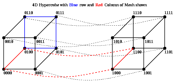
In fact it is possible to embed d = log_2 p "nonoverlapping" rings into a d-dimensional hypercube, and use them all at once to get d times the bandwidth of a single ring. The CM-2 could in fact use all d wires at each node simultaneously. These rings actually do use the same wires, but do so at different times, and so are nonoverlapping in this sense.
If there are n fish, assign n/p to each processor, and further divide these into d groups of m=n/(p*d) fish. Each group F1,...,Fd of m fish will follow a different path through the node on the algorithm. The first path will be defined by the Gray Code G(d) defined above, the second path will consist of left_circular_shift_by_1(G(d)), i.e. each address in the Gray code will have its bits left shifted circularly by 1; this clearly maintains the Gray code property of having adjacent bit patterns differ in just 1 bit. The i-th path will be left_circular_shift_by_i(G(d)). The student is invited to draw a picture of this communication pattern, which uses "all-the-wires-all-the-time", an interesting feature of the CM-2 hypercube network.
We will return to describe this software, and higher level algorithms that use it, in a later lecture.