The interfaces of these kernels have been standardized as the Basic Linear Algebra Subroutines or BLAS. The motivation for software and hardware vendors agreeing to a standard definition of these routines is their popularity: The BLAS appear in many applications (as we will see), so if vendors agree on a common interface, and supply an optimized BLAS library for each computer, then users can write programs calling the BLAS, and move their programs from one machine to another and still expect high performance.
For historical reasons, these BLAS as classified into three categories:
The Level 1 BLAS or BLAS1 operate mostly on vectors (1D arrays), or pairs of vectors. If the vectors have length n, these routines perform O(n) operations, and return either a vector or a scalar. Examples are
The Level 2 BLAS or BLAS2 operate mostly on a matrix (2D array) and a vector (or vectors), returning a matrix or a vector. If the array is n-by-n, O(n^2) operations are performed. Here are some examples.
The Level 3 BLAS or BLAS3 operate on pairs or triples of matrices, returning a matrix. Here are some examples.
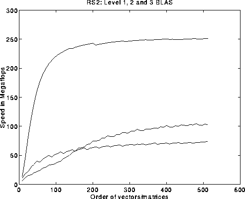
Mathematically, many these operations are essentially equivalent. For example, the dot product can be thought of as the product of a 1-by-n vector and an n-by-1 vector, and each entry of A*B is the dot product of a row of A and a column of B. So essentially any linear algebra algorithm can be expressed in terms of any of these constructs. So why distinguish among them? The answer is performance, as indicated on the following plot of BLAS performance on the IBM RS 6000/590.

The slide plots the performance in megaflops of the BLAS on the RS 6000/590, versus matrix or vector dimension. These BLAS are specially optimized by IBM to take advantage of all features of the RS 6000/590 architecture (we will discuss this in more detail later). The top curve is for matrix-matrix multiply (BLAS3), the second highest curve (for large dimension) is matrix-vector multiply (BLAS2), and the lowest curve is for saxpy (BLAS1) on the RS6000. (These plots assume the data is not initially in the cache, or fast memory.) As you can see there is potentially a big speed advantage if an algorithm can be expressed in terms of the BLAS3 instead of BLAS2 or BLAS1. The top speed of the BLAS3, about 250 Mflops, is very close to the peak machine speed of 266 Mflops. Later in the course, we will explain how to reorganize algorithms, like Gaussian elimination, so that they use BLAS3 rather than BLAS1.
Historically, the BLAS1 were invented and standardized first, because they were adequate to reach the top performance of the machines at that time (early 1970s). When they no longer reached peak performance on later machines, the BLAS2 were introduced in the mid 1980s, and the BLAS3 in 1990. As we will now explain, the reason for their performance differences is how they depend on the memory hierarchy.
To quantify our compararisons, we will use a simple model of the way the memory hierarchy works: Assume we have two levels of memory hierarchy, fast and slow, and that all data initially resides in slow memory. For each of saxpy, sgemv and sgemm, applied to vectors and matrices of dimension n, we will count
       m = number of memory references to slow memory needed just to read
           the input data from slow memory, and write the output data back
       f = number of floating point operations
       q = f/m = average number of flops per slow memory reference


              m         justification for m                          f        q
   saxpy     3*n        read each x(i), y(i) once, write y(i) once  2*n      2/3
   sgemv     n^2+O(n)   read each A(i,j) once                      2*n^2      2
   sgemm   4*n^2        read each A(i,j),B(i,j),C(i,j) once,       2*n^3     n/2
                        write each C(i,j) once
There is a clear difference in q for each level of BLAS, with BLAS3 the highest. The significance of q is this: for each word read from slow memory (the expensive operation), one can hope to do at most q operations on it (on average) while it resides in fast memory. The higher q is, the more the algorithm appears to operate at the top of the memory hierarchy, where it is most efficient. Another way to describe q is in terms of the miss ratio, the fraction of all memory references (to fast or slow memory) that ``miss'' the fast memory, and need data from the slow memory; a good problem has a low miss ratio. Assuming all input data initially resides in the slow memory, that the final result will also reside in the slow memory, and that each floating point operation involves 2 references to either fast or slow memory, we may bound
                 number of references to slow memory       m       1
   miss ratio = ------------------------------------- >= ----- = ----- .
                 total number of memory references        2*f     2*q
Thus the higher is q, the lower we can hope to make the miss ratio
by a clever choice of algorithm.
Let us use a very simple problem to illustrate why a large q means we can hope to run faster. Suppose one can do operations at 1 Mflop on data in the fast memory, and fetching data from slow memory takes 10 times longer per word. Suppose our simple algorithm is
   s = 0
   for i = 1, n
      s = s + f(x(i))
   end for
where evaluating f(x(i)) requires q-1 operations on x(i), all of which can
be done in fast memory once x(i) is available. We can assume s also resides
in fast memory. So for this algorithm m=n, and f=q*n. How fast does it run?
Assuming x(i) is initially in slow memory, this algorithm takes
time t = 10*n microsecs (to read each x(i)) plus q*n microsecs (to do q*n
flops), for a megaflop rate of f/t = q/(q+10). As q increases, this megaflop
rate approaches the top speed of 1 Mflop.
Here are some more details of our simple memory hierarchy model. We will use them to analyze several different algorithms for matrix multiplication (sgemm) in more detail, and in fact design one that uses the memory hierarchy ``optimally''.
We consider 3 implementations of matrix multiply and compute q=f/m for each.
       for i=1 to n
          {Read row i of A into fast memory}
          for j=1 to n
             {Read C(i,j) into fast memory}
             {Read column j of B into fast memory}
             for k=1 to n
                 C(i,j)=C(i,j) + A(i,k)*B(k,j)
             end for
             {Write C(i,j) back to slow memory}
          end for
       end for
Note that the innermost loop is doing a dot product of row i of A and
column j of B; this is indicated by the following figure:

Also, one can describe two innermost loops (on j and k) as doing a vector-matrix multiplication of the ith row of A times the matrix B, to get the i-th row of C. This is a hint that we will not perform any better than these operations, since they are within the inner loop. Here is the detailed accounting of memory references:
     m = # slow memory refs =   n^3     read each column of B n times
                              + n^2     read each row of A once for each i,
                                          and keep it in fast memory during
                                          the execution of the two inner loops
                              + 2*n^2   read/write each entry of C once
                            = n^3 + 3*n^2
Thus q = f/m = (2*n^3)/(n^3 + 3*n^2) ~ 2. This is the same q as for sgemv, which is no surprise as mentioned above. It is far below the upper bound of n/2. We leave it to the reader to show that reading B into fast memory differently cannot significantly improve m and q.
       for j=1 to N
           {Read Bj into fast memory}
           {Read Cj into fast memory}
           for k=1 to n
               {Read column k of A into fast memory}
               Cj = Cj + A( :,k ) * Bj( k,: )  ...  rank-1 update of Cj
           end for
           {Write Cj back to slow memory}
       end for
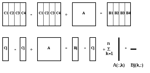
Here is a pictorial representation of the algorithm, for N=4:

The inner loop does a rank-one update of Cj, multiplying column k of A times row k of Bj. We assume that the fast memory is large enough to let us keep Bj, Cj and one column of A in it at a time; this means M >= 2*n^2/N + n, or N >= 2*n^2/(M-n) ~ 2*n^2/M, so that N is bounded below. Here is the detailed accounting of memory references:
     m = # memory refs =   n^2     read each Bj once
                         + N*n^2   read each column of A N times
                         + 2*n^2   read/write each Cj once
                       = (N+3)*n^2
Thus q = f/m = (2*n^3)/((N+3)*n^2) ~ 2*n/N.
We can increase q, and so accelerate
the algorithm, by making N as small as possible. But N is bounded below
by the memory constraint M >= 2*n^2/N + n. If we choose N as small
as possible, so that N ~ 2*n^2/M, then q ~ M/n.
Thus we need M to grow proportionally to n
to get a reasonable q. So for a fixed M, as n grows, we would expect
the algorithm to slow down. This is not an attractive property.
        for i=1 to N
           for j=1 to N
              {Read Cij into fast memory}
              for k=1 to N
                 {Read Aik into fast memory}
                 {Read Bkj into fast memory}
                 Cij = Cij + Aik * Bkj
              end for
              {Write Cij back to slow memory}
           end for
        end for
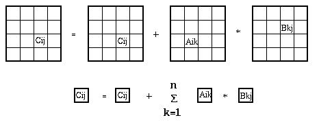
Here is a pictorial representation of the algorithm, for N=4:

Thus, the inner loop is an n/N-by-n/N matrix multiply. We assume that the fast memory is large enough so that the 3 subblocks Cij, Aik and Bkj fit in the fast memory; this means that M >= 3*(n/N)^2, or N >= sqrt(3/M)*n, so that N is bounded below. Here is the detailed accounting of memory references
     m = # memory refs =   N*n^2   read each Bkj N^3 times
                         + N*n^2   read each Aik N^3 times
                         + 2*n^2   read/write each Cij once
                       = (2*N+2)*n^2
Thus q = f/m = (2*n^3)/((2*N+2)*n^2) ~ n/N. As before, we can increase q, and so accelerate the algorithm, by making N as small as possible. But N is bounded below by the memory constraint N >= sqrt(3/M)*n. If we choose N as small as possible, so that N ~ sqrt(3/M)*n, then q ~ sqrt(M/3). Now q is independent of n, and in fact essentially optimal:
Theorem: ("I/O Complexity: the red blue pebble game", X. Hong and H. T. Kung, 13th Symposium on the Theory of Computing, ACM, 1981). Any blocked version of this matrix multiplication algorithm has q = O( sqrt(M) ), i.e. growing at most as fast as a constant multiple of sqrt(M).
There is a lot more to matrix multiplication, both theoretically and practically.
     Let M = [ m11 m12 ] = [ a11 a12 ] * [ b11 b12 ]
             [ m21 m22 ]   [ a21 a22 ]   [ b21 b22 ]

     Let
         m1 = ( a12 - a22 ) * ( b21 + b22 )
         m2 = ( a11 + a22 ) * ( b11 + b22 )
         m3 = ( a11 - a21 ) * ( b11 + b12 )
         m4 = ( a11 + a12 ) * b22
         m5 = a11 * ( b12 - b22 )
         m6 = a22 * ( b21 - b11 )
         m7 = ( a21 + a22 ) * b11

     Then
         m11 = m1 + m2 - m4 + m6
         m12 = m4 + m5
         m21 = m6 + m7
         m22 = m2 - m3 + m5 - m7
Here is the corresponding algorithm:
     M = Strassen_Matrix_Multiply(A,B,n)
        /* Return M=A*B, where A and B are n-by-n;
           Assume n is a power of 2 */
        if n=1,
            return M=A*B   /* scalar multiplication */
        else
            Partition A = [ A11  A12 ] , B = [ B11  B12 ]
                          [ A21  A22 ]       [ B21  B22 ]
                      where the subblocks Aij and Bij are n/2-by-n/2

            M1 = Strassen_Matrix_Multiply( A12 - A22, B21 + B22, n/2 )
            M2 = Strassen_Matrix_Multiply( A11 + A22, B11 + B22, n/2 )
            M3 = Strassen_Matrix_Multiply( A11 - A21, B11 + B12, n/2 )
            M4 = Strassen_Matrix_Multiply( A11 + A12, B22, n/2 )
            M5 = Strassen_Matrix_Multiply( A11, B12 - B22, n/2 )
            M6 = Strassen_Matrix_Multiply( A22, B21 - B11, n/2 )
            M7 = Strassen_Matrix_Multiply( A21 + A22, B11, n/2 )

            M11 = M1 + M2 - M4 + M6
            M12 = M4 + M5
            M21 = M6 + M7
            M22 = M2 - M3 + M5 - M7

            return M = [ M11  M12 ]
                       [ M21  M22 ]
         end
It is straightforward but tedious to show (by induction on n) that this
correctly computes the product A*B. If we let T(n) denote the number of
floating point operations required to execute Strassen_Matrix_Multiply,
then we may write down the simple recurrence:
       T(n) =    7*T(n/2)   ... the cost of the 7 recursive calls
              + 18*(n/2)^2  ... the cost of the 18 n/2-by-n/2 matrix additions
Changing variables from n to m = log_2 n changes this to a simpler
recurrence for T'(m) = T(n):
T'(m) = 7*T'(m-1) + 18*2^(2*m-2)which can be solved to show that T(n) = O( n^(log_2 (7)) ) ~ n^2.81. Strassen's method is numerically stable, but not always as accurate as the straightforward algorithm (``Exploiting fast matrix multiplication within the Level 3 BLAS'', N. Higham, ACM Trans. Math. Soft., v. 16, 1990, "Stability of block algorithms with fast Level 3 BLAS", J. Demmel and N. Higham, ACM Trans. Math. Soft., v 18, n 3, 1992). Furthermore, it requires a significant amount of workspace to store intermediate results, which is a disadvantage compared to the conventional algorithm. A long sequence of ever more complicated algorithms has appeared (``How Can We Speed Up Matrix Multiplication'' by V. Pan, SIAM Review, v 26, 1984; ``How to multiply matrices faster'' by V. Pan, Lecture Notes in Mathematics v. 179, Springer, 1984; ``Polynomial and matrix computations,'' by V. Pan & D. Bini, Birkhauser, 1994) culminating in the current record algorithm of O(n^2.376...), due to Winograd and Coppersmith ["Matrix multiplication via arithmetic progressions". In Proceedings of the Nineteenth Annual ACM Symposium on Theory of Computing, pp 1-6, New York City, 25-27 May 1987]. All but the simplest of these algorithms are far too complicated to implement efficiently. IBM's ESSL library includes an implementation of Strassen and of an algorithm by Winograd which trades some of the multiplies in the usual algorithm for more additions, which helps on some architectures. Strassen's method has also been implemented on the Cray 2 ("Extra high speed matrix multiplication on the Cray-2", D. Bailey, SIAM J. Sci. Stat. Comput., v 9, May 1988; "Using Strassen's algorithm to accelerate the solution of linear systems", D. Bailey, K. Lee, H. Simon, J. Supercomputing, v 4, 1991). A potential attraction of Strassen is its natural block decomposition; instead of continuing the recursion until n=1 (as in the above code), one could instead use a more standard matrix multiply as soon as n is small enough to fit all the data in the fast memory.
We will discuss matrix multiplication again later, for distributed memory parallel machines, where part of the algorithm design problem is to decide which processor memories store which parts of A, B and C, and which processors are responsble for computing which parts of the product A*B.