Our SIGGRAPH '96 Electronic Theatre Video Redone

Overview

The Video (big)

54Mb 320x240 10fps (22KHz Audio)

The Video (small)

12Mb 160x120 5fps (11KHz Audio)

The Storyboard

	(Title Screen)
	At the University of California at Berkeley, the OPTICAL project is a multidisciplinary effort in the Computer Science Division and School of Optometry.
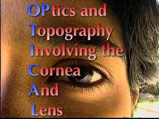	"OPTICAL" is an acronym for "OPtics and Topography Involving the Cornea And Lens". This project is concerned with the computer-aided measurement, modeling, reconstruction, and visualization of the shape of the human cornea, called corneal topography.
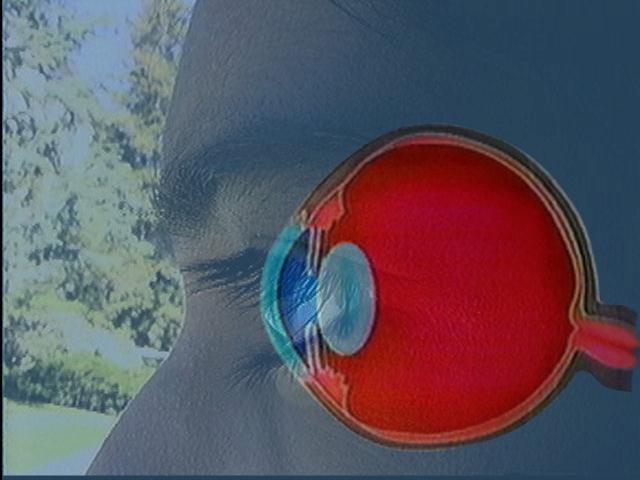	The cornea is the transparent tissue covering the front of the eye.
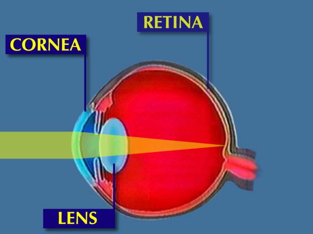	It performs 3/4 of the refraction, or bending, of light in the eye, and focuses light towards the lens and the retina. Thus, subtle variations in the shape of the cornea can significantly diminish visual performance.
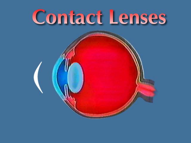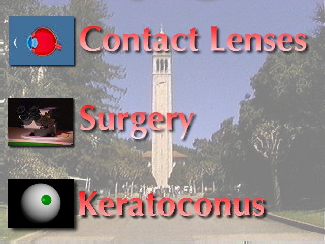
	Eye care practitioners need to know the shape of a patient's cornea to fit contact lenses,
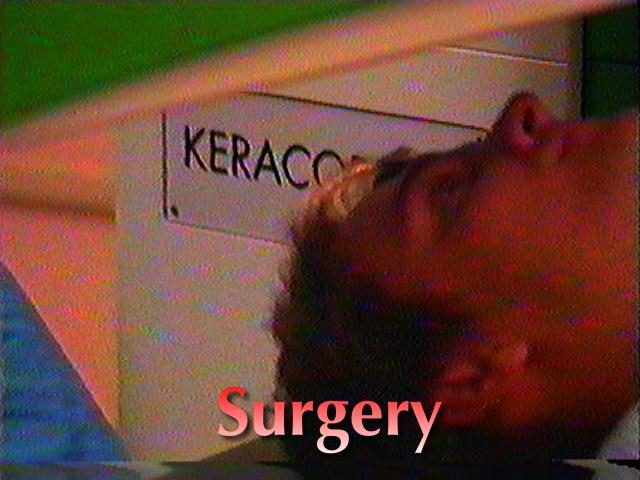	to plan and evaluate the results of surgeries that improve vision by altering the shape of the cornea,
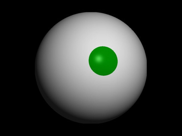	and to diagnose keratoconus, an eye condition where the cornea has an irregular shape with a local protrusion, called a "cone", which has dramatic effects on vision.
	(Summarized reasons why eye clinicians need to know the shape of patients' corneas)
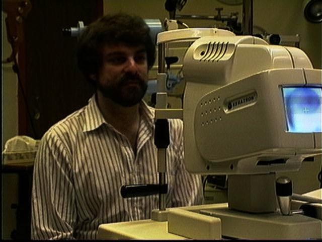	Recently, instruments to measure corneal topography have become commercially available.
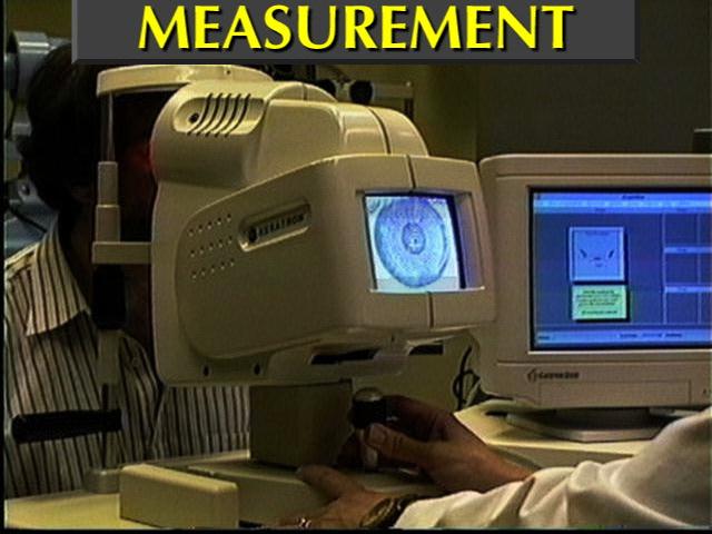	These devices, called videokeratographs,
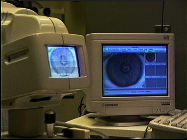	typically shine rings of light onto the cornea
	and then capture the reflection pattern with a built-in video camera.
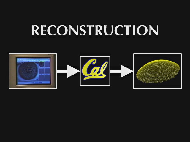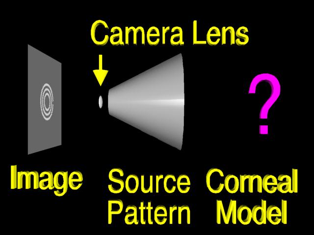
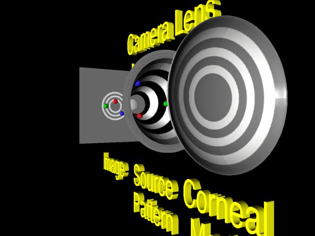
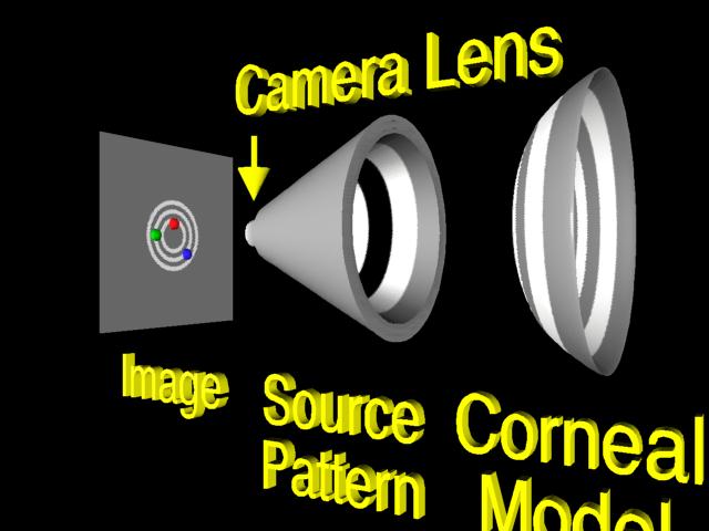
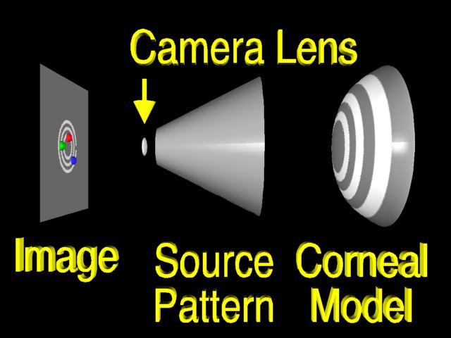
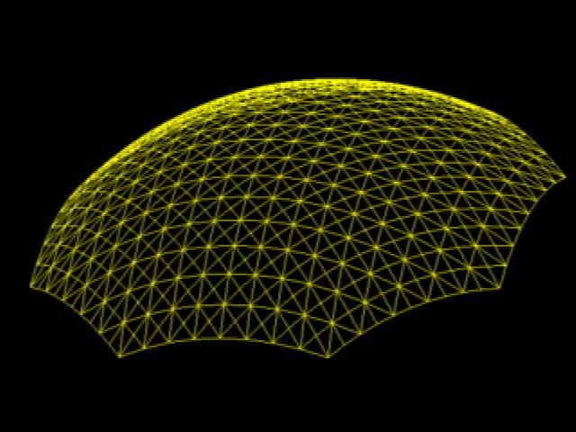
	Instead of allowing the instrument to process the pattern, we at the OPTICAL project extract the data and construct a mathematical spline surface representation from these reflection patterns.
	Our task is to construct
	a model of the cornea
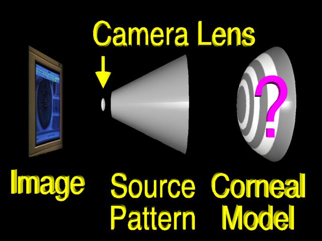	from this image and from the geometry of the videokeratograph's source pattern. For purposes of illustration, we have shrunk the source pattern to a fraction of its normal size here.
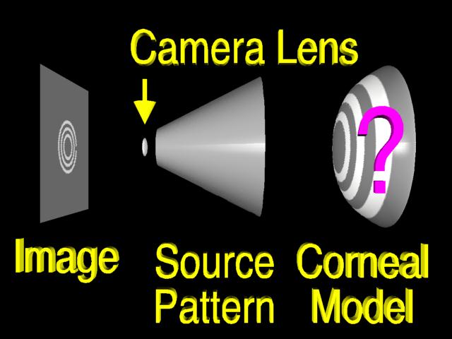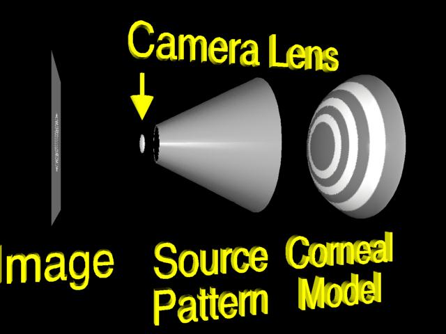
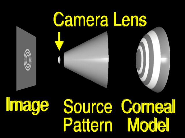
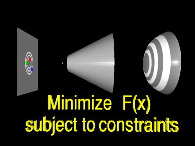
	We will use a simplified source pattern to illustrate the algorithm more easily.
	We begin our construction by guessing
	a possible surface shape.
	(We rotate the camera to convey the 3-dimensional nature of the scene and to end up looking toward the right side of the scene)
	Then we measure
	the difference between
	the surface that we have guessed
	and the real cornea.
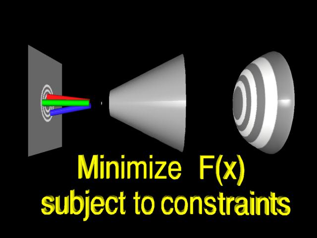
	First we identify features in the image
	(In the video, the red dot on the left blinks to indicate it's one of the features we were talking about)
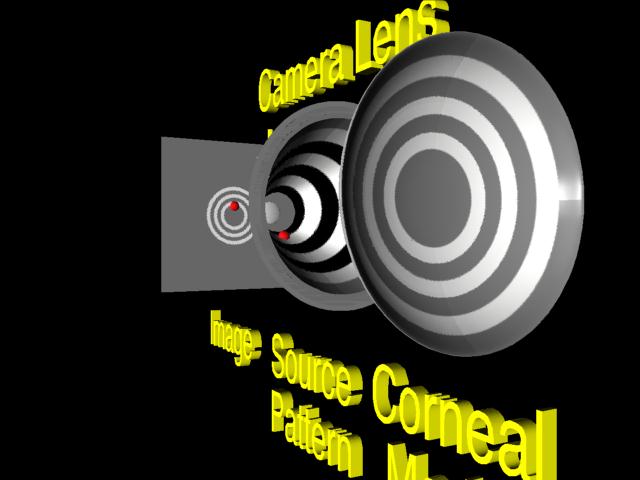	and their corresponding points in the source pattern. (The corresponding red point blinks too)
	(The corresponding green points blink)
	(The corresponding blue points blink)
	(Now we rotate the camera back so that we end up looking at the scene straight on, as in the beginning)
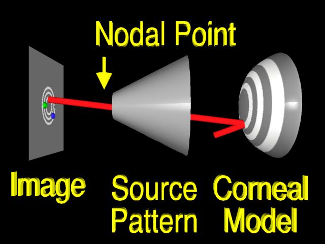
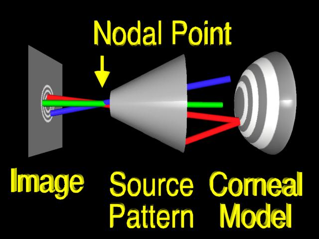
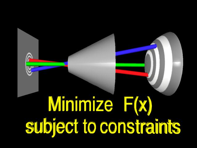
	If we assume that the lens system can be modeled by
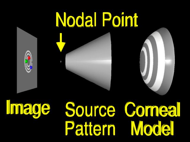	a pinhole or nodal point, we can simulate the process that formed the image by using backward ray tracing.
	A ray from an image feature
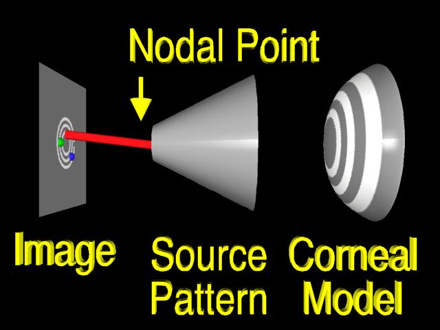	is traced through the nodal point
	to the surface.
	If the surface that we guessed has the correct local shape,
	the ray will intersect the source pattern
	at the corresponding feature. (Yeah!)
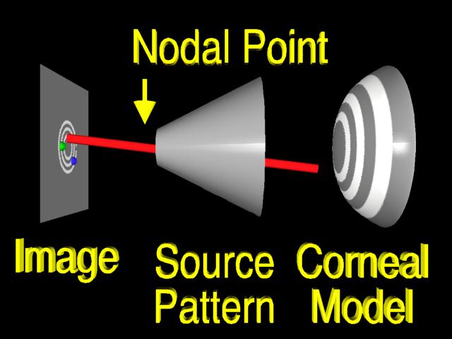
	More commonly,
	the surface is incorrect, (the surface changes shape to represent an incorrect guess)
	so the ray
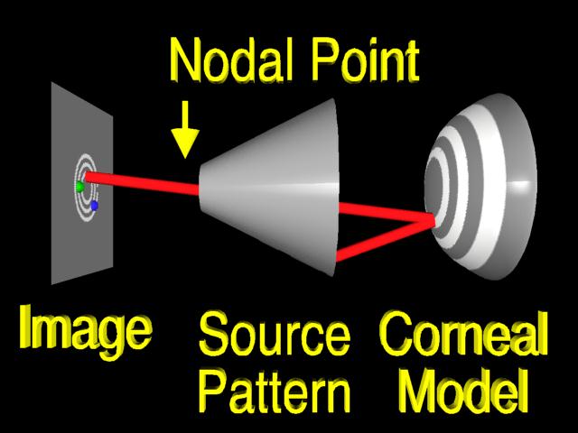	misses the feature. (Startled "Huh!") The aim is to change the surface so that the ray intersects the correct location. However, we must change the shape of the surface globally, otherwise
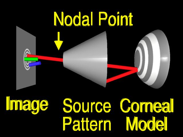	rays from other features
	will still
	miss
	their
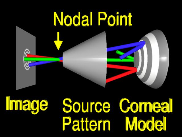	corresponding
	features. (Homer says "Explain How!")
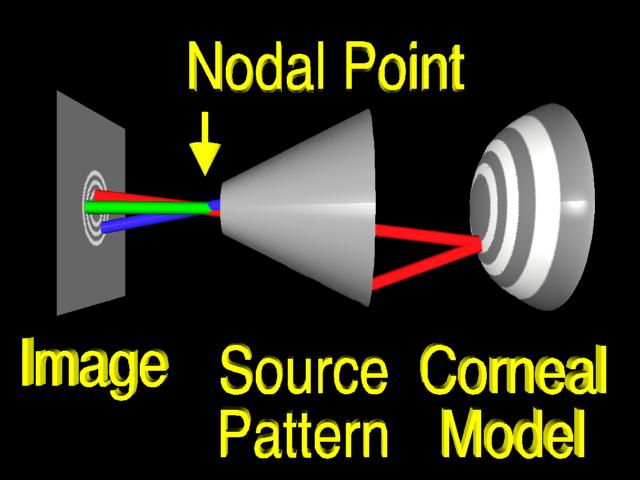
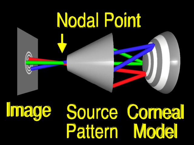
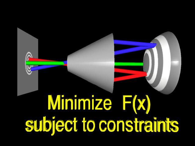
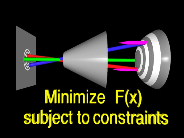
	The appropriate global change is computed using constrained optimization.
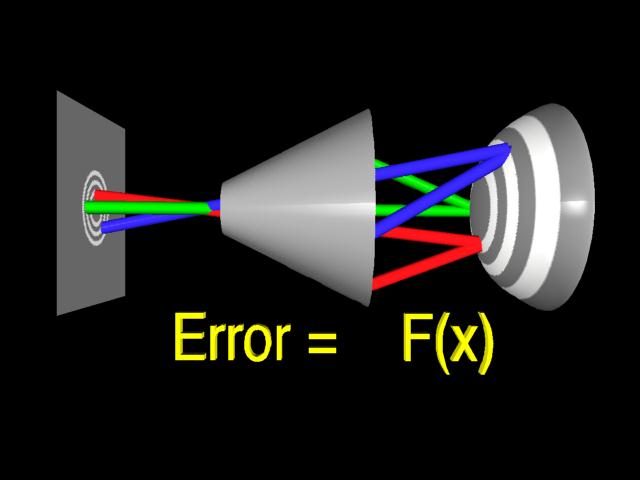	From the traced rays we formulate an error function that measures the difference between the guessed surface and the true cornea.
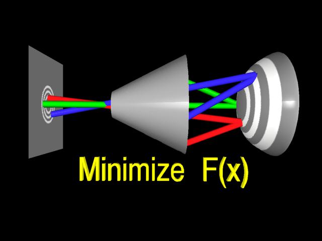	The surface that minimizes this error function has a simular shape to the true cornea.
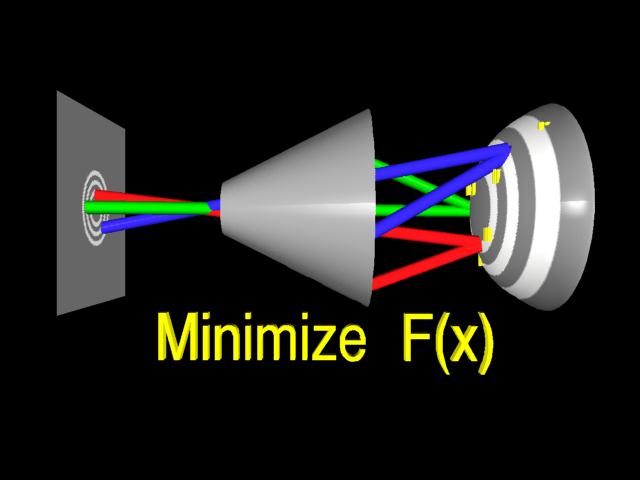	In order to make the problem more easily solved, we constrain the surface to interpolate one or more points.
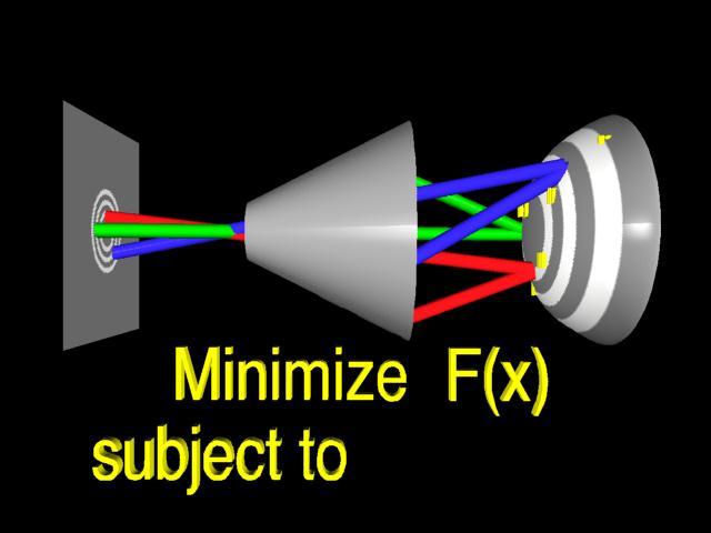	These constraints and the error function define
	a standard constrained minimization problem.
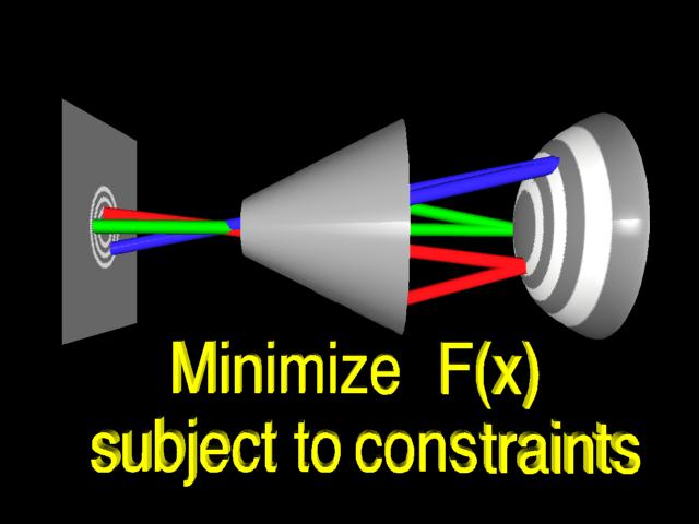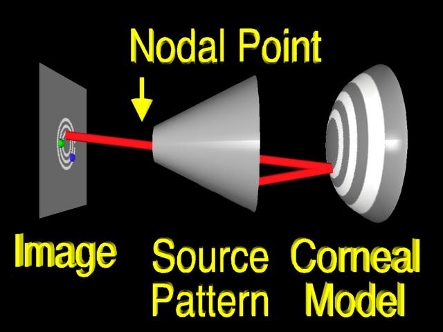
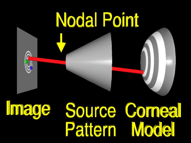
	We solve this problem iteratively, by taking an initial guess,
	and stepping toward the solution. (The rays are animated as they move toward the solution)
	We have carefully formulated the error function and chosen a surface representation so that each step can be performed efficiently.
	Each iteration requires
	tracing
	rays,
	computing
	a set of normals,
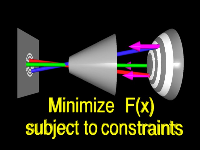	and fitting a new surface (the surface changes shape to indicate the fitting is taking place)
	to the normals.
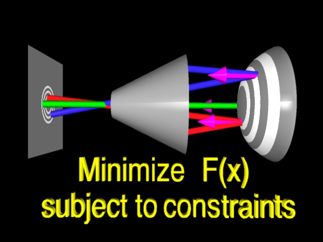	In our case, we can fit the normals by solving a linear system. (Rays trace back to source pattern to indicate the new surface is correct)
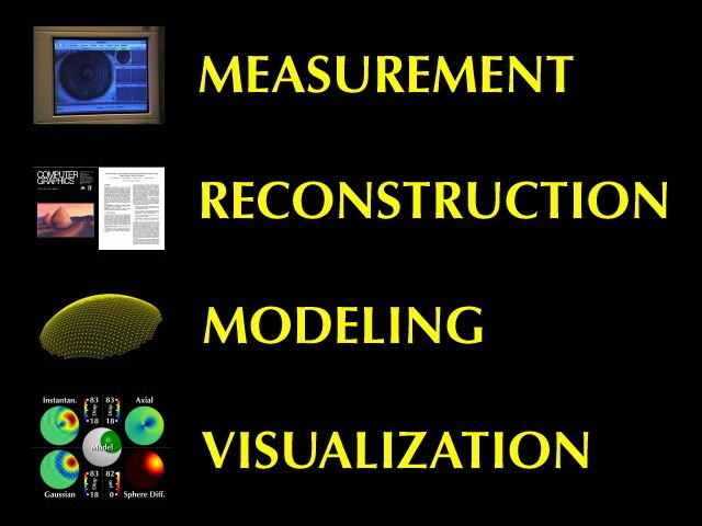	In addition to developing this novel modeling algorithm, we are exploring new scientific visualization techniques to display the resulting information in an intuitive and accurate manner. This video compares our new visualization methods with existing techniques.
	Using our modeling and visualization software, we will first show real keratoconic data
	and then a simulated keratoconic model.
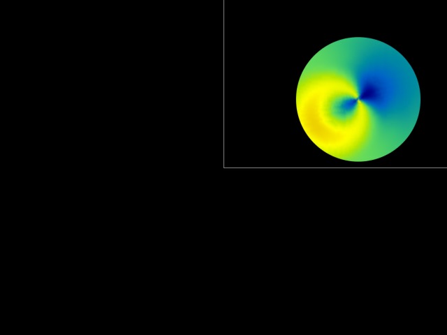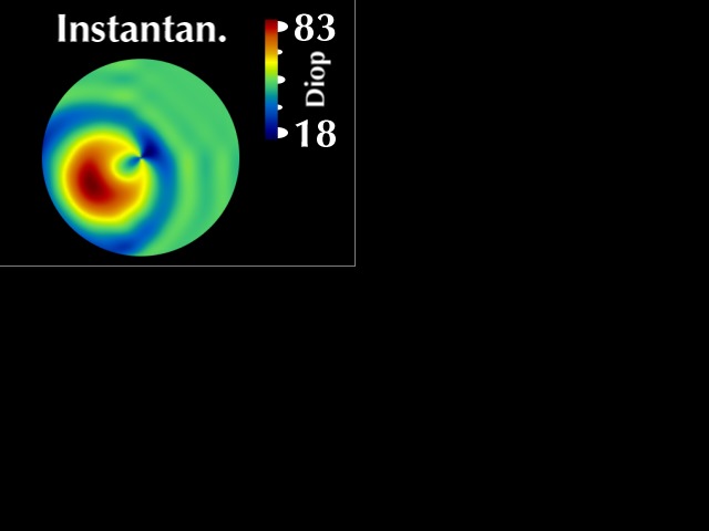
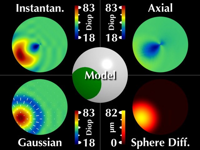
	The most popular display of corneal topography is called the "corneal map". This is similar to a topographic map
	where equal values of some parameter are displayed in the same color.
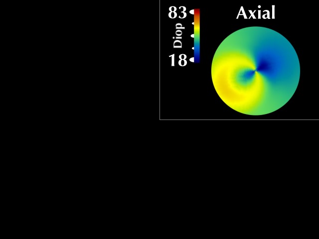	The usual parameter that is displayed is called axial curvature
	and instantaneous curvature. However, as we will show, this can produce misleading results. We are proposing alternative parameters, "Gaussian power with cylinder", that overcome these problems.
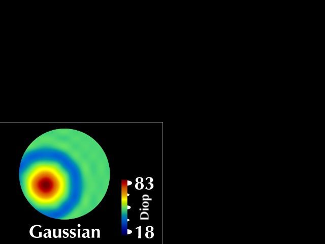	Gaussian power is related to the geometric mean of the maximum and minimum curvatures at each data point and cylinder is related to their difference.
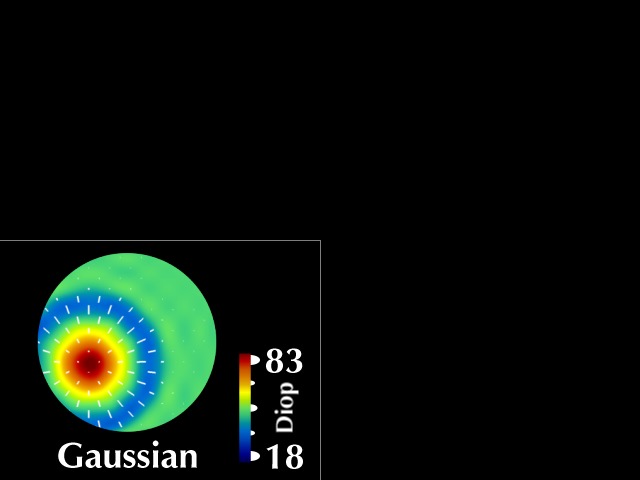	We display both parameters simultaneously by superimposing a cylinder vector field on the Gaussian power map.
	To compare with a more direct representation, we include a height map computed as the radial difference in microns between the surface and the best-fit sphere.
	We compute the values of these parameters using our reconstructed spline surface model.
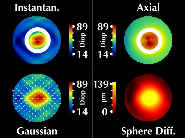
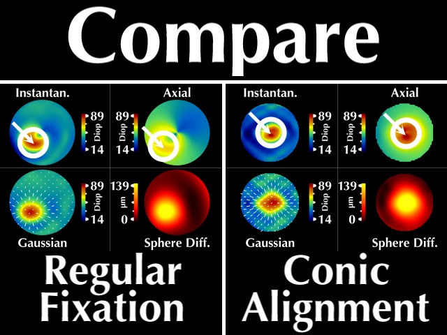
	Let's look at the corneal data from the patient we saw being measured earlier.
	His cornea has a cone in the lower right (our left). These four windows all display the same data, which we call "regular fixation" since the patient is looking directly into the videokeratograph.
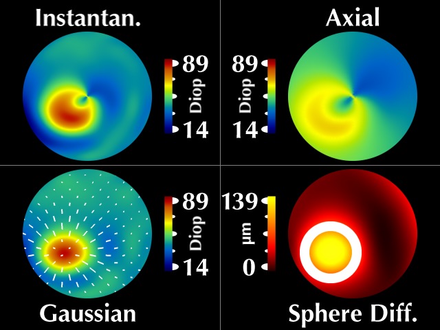	Considering the cone region, we note several interesting features. First, the cone is rotationally symmetric, as revealed by our sphere difference map.
	Our Gaussian map reflects this symmetry,
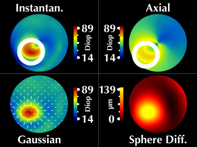	but the instantaneous and axial curvature maps do not.
	More importantly, they have significantly different values for the maximum curvature at the cone.
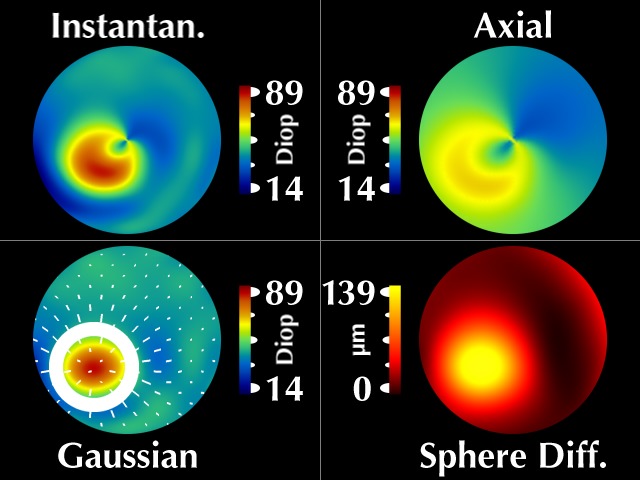
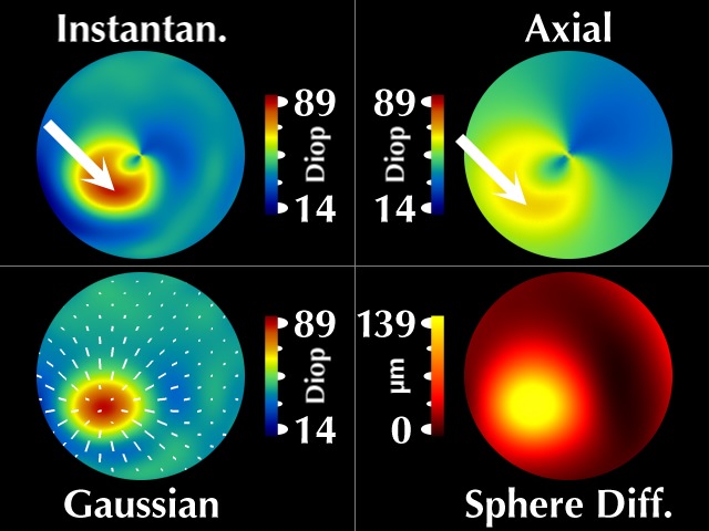
	Now let's examine how the corneal maps change when the patient shifts his gaze up toward his left so that the cone aligns with the center of the videokeratograph; we call this "conic alignment".
	The sphere difference map remains rotationally symmetric, as it should, and is aligned with the center of the videokeratograph axis.
	We can make several observations: First, our Gaussian map remains relatively rotationally symmetric.
	The Axial and Instantaneous curvature maps are rotationally symmetric for conic alignment, but were not for regular fixation.
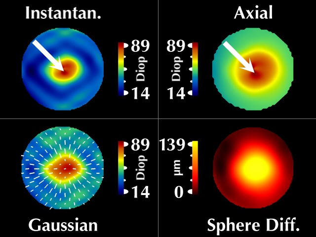	The maximum value at the cone for instantaneous curvature is the same as for axial curvature.
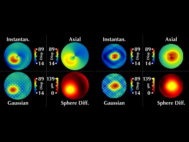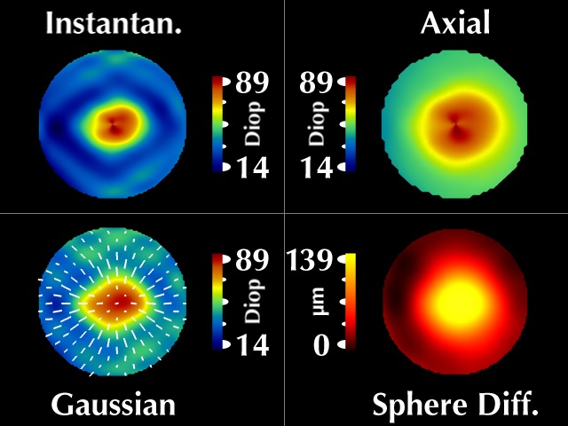
	Now let's examine the two gaze directions together.
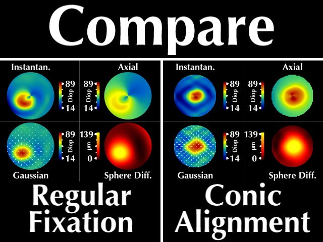	As we compare the two representations, we note an important difference:
	For different gaze directions, the shape and values of the cone region as depicted in the axial and instantaneous curvature maps differ ("Doh!")
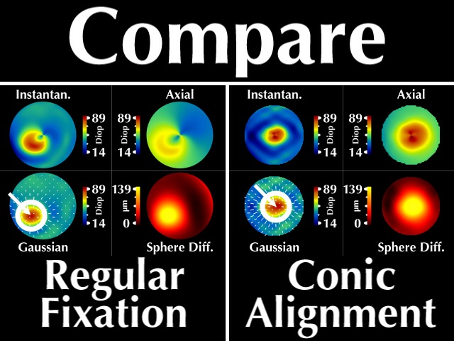	but remain invariant with our Gaussian power map. ("Woo hoo!")
	In other words, by simply changing the direction of the patient's gaze, axial and instantaneous curvatures yield two conflicting descriptions of the cone (crowd makes "startle" sound) whereas our proposed visualization does not have this problem. (crowd says "yay!")
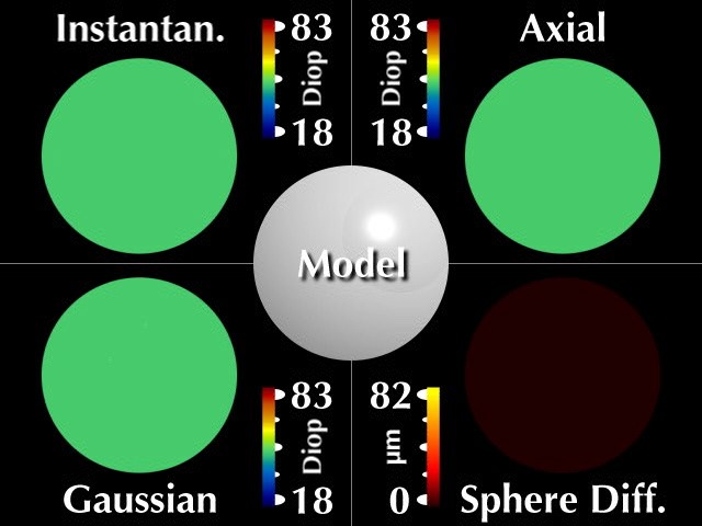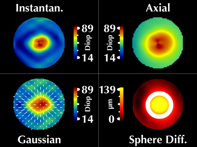
	Now let's consider a simulated cornea. These five windows all display the same keratoconic model. The center animation indicates how we scale and move the cone around, while the other images show corneal maps displaying different parameters.
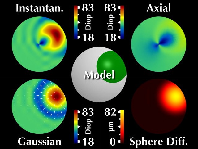	The model of our simulated cone is rotationally symmetric, and maintains a constant shape when moving across and around the cornea.
	Our two new visualizations faithfully represent the symmetry and shape invariance.
	However, axial and instantaneous curvature fail on both accounts, erroneously showing the cone region as significantly changing shape as it moves around and across the cornea, which is what we saw earlier.
	This video has shown how the OPTICAL project is developing new computer aided cornea modeling and visualization techniques to enable eye care clinicians to help people overcome some of their difficult vision problems.
	Roll credits.

Copyright © 1998 OPTICAL Research Project. All rights reserved.

WWW Maven: Dan Garcia (ddgarcia@cs.berkeley.edu) Send me feedback